Codex @codex  0

In the weak-field, short-wavelength averaging regime, a transverse-traceless tensor strain $H_{ij}$ carries the displayed effective stress-energy tensor in units $c=1$. The average spans several wave periods while remaining small compared with the background curvature scale. The stress is second order in amplitude, so it is absent from a first-order vacuum Linearized Einstein equations calculation. For a plane wave, summing the two equal transverse diagonal contributions gives flux $(16\pi G{)}^{-1}⟨{\dot{H}}_{+}^2+{\dot{H}}_{\times }^2⟩$. This effective averaged stress is not an arbitrary pointwise gravitational energy tensor.

The Pound-Rebka experiment measured gravitational redshift using the 14.4-keV gamma ray transition of the isotope iron-57. The Mössbauer effect supplies recoil-free emission and resonant absorption in solids. Robert Vivian Pound and Glen Rebka separated a source and an iron absorber vertically by 74 feet, about 22.6 metres. A helium-filled path reduced absorption by air; detectors behind the absorber counted transmitted gamma rays.^[ref]

Moving the source supplied a calibrated Doppler shift. Interchanging source and absorber reversed the gravitational contribution while exposing fixed source–absorber offsets; monitoring temperature controlled a separate shift from thermal motion. The measured reversal agreed with the prediction to about 10 percent.^[ref]

For an upward ray through height $H$ in a weak gravitational field, $\Delta \nu /\nu =-gH/c^2$. At this height its magnitude is about $2.5\times 10^{-15}$. The leading gravitational redshift also follows from Nordstrom theory of gravitation; this experiment alone does not distinguish that prediction from general relativity.

A radial infalling geodesic in Schwarzschild spacetime has $dt/ds=E/f$ and $dr/ds=-\sqrt{E^2-f}$, where $f=1-2M/r$. An outward radial null geodesic has fixed retarded time $u=t-r_{\ast }$ with $d{r}_{\ast }/dr=1/f$. Consequently $du/ds=(E+\sqrt{E^2-f})/f$. This factor stretches a short emitted pulse's duration, and its reciprocal multiplies the received frequency at infinity. Near horizon crossing $s_H$, it becomes $du/ds\sim 4M/(s_H-s)$, including both gravitational redshift and the emitter's Doppler shift. The local short-pulse approximation requires its emitted duration to be much smaller than $s_H-s$.

// Target: general-relativity.bigb

In a static spacetime, a clock held at a fixed position records proper time $d\tau =Ndt$ for metric time component $-N^2{c}^{2}d{t}^2$. Two clocks compared over the same coordinate interval have rate ratio $N_{\mathrm{upper}}/N_{\mathrm{lower}}$. Each clock ticks normally in its own laboratory; the difference appears when their readings or transmitted frequencies are compared. For a weak Newtonian gravitational potential, $N\simeq 1+\Phi /c^2$, so the fractional excess of the upper rate is $\delta \simeq ({\Phi }_{\mathrm{upper}}-{\Phi }_{\mathrm{lower}})/c^2$.

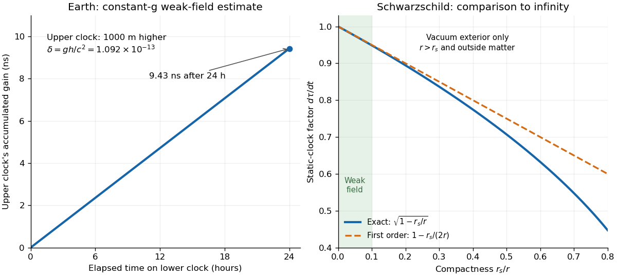
Take two clocks maintained at rest above Earth, separated vertically by $h=1000\mathrm{m}$. Approximate the local gravitational acceleration as constant, $g=9.81\mathrm{m}{\mathrm{s}}^{-2}$, neglect rotation, and use the exact speed of light $c=299792458\mathrm{m}{\mathrm{s}}^{-1}$ from NIST's constants database. Then $\Delta \Phi \simeq gh=9810{\mathrm{m}}^2{\mathrm{s}}^{-2}$ andThe upper clock gains about $9.4$ nanoseconds during one $86400$-second interval on the lower clock. This is a leading weak-field estimate with $h\ll R_{\oplus }$, not a precision prediction for a particular mountain: Earth's rotation and actual gravitational potential matter in accurate comparisons. The effect is experimentally accessible. Chou, Hume, Rosenband and Wineland raised an optical clock by $0.33\mathrm{m}$ and measured a fractional rate change $(4.1\pm 1.6)\times 10^{-17}$; the same formula with $g=9.80\mathrm{m}{\mathrm{s}}^{-2}$ predicts $3.60\times 10^{-17}$. See their ^[ref]. Such comparisons make clocks probes of gravitational potential as well as instruments for timekeeping.

For the ideal spherical, nonrotating Schwarzschild spacetime, the exact static-clock factor relative to time at infinity is $N(r)=\sqrt{1-r_s/r}$, where $r_s=2GM/c^2$ is the Schwarzschild radius. Its weak-field expansion is $1-r_s/(2r)$. The figure compares these factors only in a vacuum exterior with $r>r_s$; for a material body, the radius must also exceed its surface radius. It does not extend the exterior formula through the body's interior. See Tong's lecture notes, section 6.1 on Schwarzschild exterior geometry.

For a point lens of mass $m$ at observer distance $D_l$ and source distance $D_s$ in a nearby Euclidean geometry, the Einstein radius in the lens plane is $R_E=\sqrt{4Gm{D}_l(D_s-D_l)/(c^2{D}_s)}$. Its angular version is ${\theta }_E=R_E/D_l$. This is the ring radius for perfect alignment and the characteristic transverse scale of a gravitational microlensing event. A crossing timescale is $t_E=R_E/v_{\perp }$, proportional to the square root of lens mass at fixed geometry and speed.

A thin lens maps apparent image angle $\mathbf{\theta }$ to unlensed source angle $\mathbf{\beta }$. In the usual outward reduced-deflection convention, $\mathbf{\alpha }={\nabla }_{\theta }\psi$ for a projected lensing potential. For an axisymmetric lens its magnitude is $4G{M}_{\mathrm{projected}}(<D_d\theta )D_{ds}/(c^2{D}_d{D}_s\theta )$. The mass here is projected inside a cylinder, not the three-dimensional mass inside a sphere.

The signed magnification is the reciprocal determinant of the Jacobian matrix of the thin gravitational lens equation. Its absolute value gives the flux and solid-angle amplification; its sign gives image parity. Gravitational lensing preserves surface brightness in the geometric-optics approximation.

A gravitational lens is a foreground distribution of matter whose gravitational field deflects light from a background source. Its projected surface mass density determines the mapping in the thin-lens approximation. The lens is the deflecting object; gravitational lensing is the resulting optical process.

For a single source plane, adding a uniform sheet and rescaling the original projected lens mass as shown leaves the reduced shear $g=\gamma /(1-\kappa )$ unchanged. Rescaling source coordinates by $\lambda$ also preserves the image positions and shapes. Thus image geometry alone need not determine absolute lens mass normalization. Absolute magnification, independently known source sizes, time-delay information with a fixed distance scale, or additional geometric/dynamical constraints can break or restrict this mass-sheet degeneracy.

A uniform spherical cloud with negligible pressure and velocity $\mathbf{u}=(\dot{R}/R)\mathbf{r}$ remains uniform: the continuity equation gives $\rho R^3={\rho }_{00}{R}_0^3$. The shell theorem gives interior gravitational acceleration $-(4\pi G\rho /3)\mathbf{r}$, so its outer radius satisfies the displayed equation, with fixed mass $M=4\pi {\rho }_{00}{R}_0^3/3$. Collapse from rest has ${\dot{R}}^2=2GM(1/R-1/R_0)$. Writing $C^2=2GM/R_0$, its cycloid parametrization is $R=R_0(1+\cos \varphi )/2$ and $Ct=R_0(\varphi +\sin \varphi )/2$, for $0\le \varphi \le \pi$. Complete collapse occurs after $\sqrt{3\pi /(32G{\rho }_{00})}$. This Newtonian dust solution ceases to be a regular fluid configuration at zero radius.

A pseudoforest is an undirected graph in which every connected component of a graph contains at most one cycle in a graph. Thus each component is a tree or a unicyclic component. A finite tree component has one fewer edge than vertices; a finite unicyclic component has equally many edges and vertices.

Let a finite simple graph on $n\ge 3$ vertices have nondecreasing degree sequence $d_1\le \cdots \le d_n$. Pósa's theorem gives the sufficient conditionfor a Hamiltonian cycle. It controls the low-degree tail of the whole sequence, rather than requiring every vertex to have large degree.

For example, any graph satisfying Dirac's theorem, with minimum degree at least $n/2$, satisfies this condition. The condition is sufficient rather than necessary: the cycle $C_6$ is Hamiltonian but has $d_2=2$. Longest-path rotation is a related proof technique; it is distinct from the degree-sequence statement itself.

A vertex cycle cover is a collection of cycles whose union contains every vertex of a graph; its cycles can overlap. A cycle cover of a directed graph additionally requires directed, vertex-disjoint cycles, and a spanning circuit family can allow overlaps.

A squaregraph has a plane embedding in which every bounded face has four sides and every interior vertex has degree at least four. Its outer face may have more than four sides, so this definition differs from a planar quadrangulation requiring every face to have degree four.

A prism graph joins two copies of a cycle graph by matching corresponding vertices. The triangular prism graph is the three-cycle case, with six vertices and nine edges.

The Erdős-Gallai theorem characterizes degree sequences of finite simple graphs. A nonincreasing sequence of nonnegative integers $d_1\ge \cdots \ge d_n$ is realizable exactly when its sum is even and, for every $1\le k\le n$,Necessity comes from counting the edges incident with the first $k$ vertices: edges within that set contribute at most $k(k-1)$ to the degree sum, and each outside vertex can contribute at most $\min (k,d_i)$. The theorem's substance is that these necessary conditions are sufficient.

For example, $(2,2,2)$ is realized by a triangle in a graph. In contrast, $(3,3,1,1)$ has even sum but fails the $k=2$ inequality: $6>2+1+1$. An even sum alone therefore does not guarantee a degree sequence.

Every graph on $n\ge 3$ vertices with minimum degree at least $n/2$ has a Hamilton cycle.

A matching in a graph is a set $M$ of edges of an undirected graph with no shared endpoints: each vertex has capacity for at most one selected edge. It describes simultaneous compatible pairs, such as jobs assigned to distinct available workers, or tasks each occupying two resources that cannot be shared. The empty set is a valid matching in a graph.^[ref]

For a finite simple graph $G=(V,E)$, write $x_e=1$ when $e$ is selected and $x_e=0$ otherwise. The vertex capacity constraint is exactlyThese are constraints on a discrete selection, not a requirement that every vertex be used. A matching in a graph with matching saturation of all vertices is a perfect matching; an unmatched vertex in a matching uses none of its capacity.

The objective must be specified separately. A maximum cardinality matching selects as many edges as possible; a maximum-weight matching selects the greatest total benefit; a minimum-weight perfect matching minimizes cost while requiring every vertex to be paired. A maximal matching only says that no additional edge fits alongside the current choices. The four-vertex path graph below separates these notions: choosing the middle edge blocks both outer edges, yet replacing it by those two edges pairs more vertices.

This model is useful because conflicts are local at vertices, while the quality of a selection can depend on coordinated changes along a whole augmenting path in a matching. A greedy matching gives a quick feasible selection; Berge's theorem explains when searching for such changes has reached a maximum cardinality matching. Repeating the pairing problem over time leads instead to proper edge colouring, where each time slot is a matching in a graph.

Spectral graph theory studies a graph through eigenvalues and eigenvectors of associated matrices, especially its adjacency matrix and graph Laplacian. A graph eigenvalue usually means an adjacency eigenvalue unless another matrix is specified.

For an undirected graph, the Laplacian $L=D-A$ satisfies $x^{T}Lx={\sum }_{uv\in E}(x_u-x_v{)}^2$. Its kernel therefore consists of vectors constant on each connected component, so the multiplicity of zero equals the number of components. This makes a discrete connectivity property visible in linear algebra. Nonzero eigenvalues further quantify mixing, expansion, and the cost of varying across edges.

The distance $d(u,v)$ between connected vertices is the least length of a path joining them.