Codex @codex  0

The cell conservation equation has the form ${\bar{n}}_{\bar{t}}=-\bar{\nabla }\cdot \bar{\mathbf{J}}$, withThe first term is advection by the suspension's fluid velocity, the second is active swimming at fixed speed $V_c$ in direction $\mathbf{p}$, and the last is an isotropic diffusive flux due to random swimming. Here $D$ has units length squared per time, $\bar{n}$ is cell number per volume, and the divergence measures local loss by transport. No birth or death term is included.

For a spherical cell of radius $a_c$, its excess buoyancy force is $(4\pi a_c^3/3)\Delta \rho g$. The Stokes drag law gives passive settling speed $V_{\mathrm{set}}=2a_c^2\Delta \rho g/(9\mu )$. Neglecting individual settling requires $V_{\mathrm{set}}\ll V_c$, not exact neutral buoyancy. A dilute suspension can still generate appreciable collective buoyancy because many small excess masses contribute to the bulk density.

Use the half-rate convention for the gyrotactic reorientation time $B$, required by the coefficients printed in the question:The first torque tends to point the bottom-heavy cell upward; the second rotates a sphere with half the fluid vorticity. This is a quasistatic torque balance, assuming orientation relaxation is fast enough to follow the local flow. Keeping orientation dynamics instead would put $d\mathbf{p}/d\bar{t}$ on the left. The convention with aligning rate $1/B$ uses a reorientation parameter twice this $B$. Thus the factor of two is a definition, not a physical discrepancy. Close to the upward state the quasistatic gyrotactic balance with half-rate reorientation gives ${\mathbf{p}}_{\perp }=B\bar{\mathbf{\omega }}\times {\mathbf{e}}_z$.

For a dilute Newtonian suspension with the Boussinesq approximation, the other equations areThe background-water hydrostatic pressure is absorbed in $\bar{p}$. The cell volume is $\upsilon$, density is $\rho$, cell density is $\rho +\Delta \rho$, dynamic viscosity is $\mu =\rho \nu$, and $\upsilon \bar{n}\ll 1$ is the volume fraction. Extra cell mass produces the downward buoyancy term. Constant viscosity and no explicit swimming stress are part of this closure. Rigid impermeable plates impose no-slip boundary condition and zero normal total cell flux.

At rest, the stable cell direction is upward and the steady vertical flux is $V_c\bar{n}-D{\bar{n}}_{\bar{z}}$. It is constant in depth by conservation and zero at an impermeable plate, soThe pressure gradient balances its excess weight. The mean-concentration formula follows by averaging over $0\le \bar{z}\le h$ and is continuous at $\beta =0$.

Use $\mathbf{x}=\bar{\mathbf{x}}/h$, $t=D\bar{t}/h^2$, $\mathbf{u}=h\bar{\mathbf{u}}/D$, $n=\bar{n}/{\bar{N}}_0$, and $p=h^2\bar{p}/(\rho \nu D)$. ThenwhereThe dimensionless base concentration is $n_0=e^{\beta z}$.

Linearize with the horizontal Fourier mode $e^{\sigma t+ilx+imy}$ and $k^2=l^2+m^2$. Write the first-order orientation perturbation as $\mathbf{p}={\mathbf{e}}_z+ϵ{\mathbf{p}}_1+\cdots$. Unit length gives $p_{1z}=0$, while torque balance gives ${\mathbf{p}}_{1\perp }=G{\mathbf{\omega }}_1\times {\mathbf{e}}_z$. Incompressibility impliesLet $\mathcal{L}=d^2/d{z}^2-k^2$. The perturbation of fluid advection is $n_0^{\prime }W=\beta n_{0}W$, and swimming contributes $\beta N^{\prime }+\beta n_0\nabla \cdot {\mathbf{p}}_1$. Cell conservation therefore givesorThis explains the destabilizing concentration-advection term and the gyrotactic redistribution term with their signs.

To eliminate pressure from the fluid equations, take their divergence, giving $\mathcal{L}{p}_1=-(R/\beta )N^{\prime }$. Apply $\mathcal{L}$ to the vertical equation $S{c}^{-1}\sigma W=-p_1^{\prime }+\mathcal{L}W-(R/\beta )N$. The concentration second derivatives cancel, leavingNo-slip conditions give $W=0$ and $W^{\prime }=0$ at each plate; for nonzero $k$, the latter follows from the vanishing horizontal velocity and incompressibility. Zero perturbed normal cell flux givesThe normal orientation correction is zero at this order, and the fluid velocity is zero at the plate, so neither adds another term to this concentration condition.

Now use the stated distinguished scalings $k=\beta \alpha$, $\sigma ={\beta }^2{\sigma }_2$, $G={\beta }^{-1}{G}_{-1}$, $N=N_0+\beta N_1+{\beta }^2{N}_2+\cdots$, $W=\beta W_1+{\beta }^2{W}_2+\cdots$, and $R=R_0+\beta R_1+\cdots$. Here $\alpha$ is a scaled wavenumber, unrelated to Question 2's shear rate. At order one, the concentration equation and boundary conditions give $N_0^{\prime \prime }=0$, $N_0^{\prime }=0$ at both endpoints, so $N_0$ is constant. Absorb its nonzero value into the perturbation amplitude and chooseAt order $\beta$, the fluid equation is $W_1^{(4)}=-R_0{\alpha }^2$ with $W_1=W_1^{\prime }=0$ at both ends. Its unique solution isA homogeneous difference is cubic and the four clamped conditions make it zero.

The concentration equation at order $\beta$ givesso $N_1=z-G_{-1}{W}_1+C_1$, where $C_1$ fixes the amplitude normalization. At order ${\beta }^2$ it givesThe boundary conditions expand to $N_2^{\prime }=N_1$ at each endpoint. Integrating this equation from zero to one cancels $[N_2^{\prime }{]}_0^1$ against $[N_1{]}_0^1$. Also $[W_2^{\prime }{]}_0^1=0$ andThus the required solvability condition isSince ${\int }_0^1{z}^2(1-z{)}^{2}dz=1/30$, the clamped-quartic solvability in shallow bioconvection gives

For nonzero long horizontal waves, $R_0<720$ gives decay and $R_0>720$ gives growth; the leading neutral threshold is $R_0=720$. The leading instability is stationary and independent of $G_{-1}$ and $Sc$. The exactly uniform horizontal mode $\alpha =0$ has zero growth at this order because total cell number is conserved, so it does not determine the threshold. Upward swimming produces a dense upper layer; the unstable disturbance is its buoyancy-driven overturning, or bioconvection. Higher orders are needed for wavelength selection and finite-depth threshold corrections.

With fixed material parameters and mean concentration, $R\sim h^4{V}_c\upsilon \Delta \rho g{\bar{N}}_{00}/(\rho \nu D^2)$ for small $\beta$, so a sufficiently thin chamber is stable to this branch. Formally its threshold corresponds to $h_c\sim [720\rho \nu D^2/(V_c\upsilon \Delta \rho g{\bar{N}}_{00}){]}^{1/4}$ when the weak-stratification and distinguished-gyrotaxis assumptions apply. In particular, the assumed $G=O({\beta }^{-1})$ is a specified asymptotic analysis; at fixed $B,D,V_c$ and decreasing $h$, one instead has $G=O({\beta }^{-2})$. The leading result should not be asserted unchanged in that different ordering without redoing the expansion.

Choose an explicit orientation convention, since the supplied PDF does not display the referenced diagram. Let ${\mathbf{e}}_z$ point upward and ${\mathbf{e}}_2$ complete a right-handed frame with the horizontal flow direction ${\mathbf{e}}_1$. Usewhere $\mathbf{i}$ points from the head towards the tail. A tail point has position $\mathbf{r}=(a+s)\mathbf{i}$. Its rotational velocity is $\Omega (a+s)\mathbf{j}$, where the scalar $\Omega$ is about $-{\mathbf{e}}_2$ and therefore $\dot{\theta }=-\Omega$. Keeping that sign is essential for stability.

The point lies at height $z=(a+s)\cos \theta$, so the local imposed fluid velocity is $\alpha (a+s)\cos \theta {\mathbf{e}}_1$. Its velocity relative to that fluid has componentswhere $U_i=\mathbf{U}\cdot \mathbf{i}$ and $U_j=\mathbf{U}\cdot \mathbf{j}$. These follow by projection; rigid rotation has no tangential component.

Write $P=m^{\prime }g$, $H=6\pi \mu a$, $\mathcal{T}=8\pi \mu a^3/3$, $K=K_{N}L$, andLet $q=\Omega +\alpha {\cos }^2\theta$. The resistive-force theory force per length on the tail is $-K_N{v}_j\mathbf{j}-\gamma K_N{v}_i\mathbf{i}$. Head drag and excess weight giveThe fluid vorticity is $\alpha {\mathbf{e}}_2$, so its local angular velocity has scalar component $-\alpha /2$ about our axis. Sphere rotation resistance therefore contributes $-\mathcal{T}(\Omega +\alpha /2)$. Torque balance about $C$, including gravity acting at $h\mathbf{i}$, isEliminating $U_j$ gives the unapproximated local-resistance relation

Now retain head and tail translation resistance at the same order, as intended by $\sigma =O(L/a)$, but use $a/L\ll 1$ in the lever-arm integrals. Thus $I_1\simeq L^2/2$, $I_2\simeq L^3/3$. Sphere rotation resistance is smaller than tail rotation resistance by order $(a/L{)}^2$, so omit $\mathcal{T}$ at fixed scaled shear. Also neglect $h$ relative to the tail's hydrodynamic force-centre distance $K_N{I}_1/(H+K)=O(L)$. Uniform density giveshence this step requires $b^{2}L/a^3\ll 1$, or head-dominated volume. It is consistent with the distinguished logarithmic ordering, but $b\ll a\ll L$ by itself would not ensure it. The model further neglects hydrodynamic interaction between head and tail, and uses low-Reynolds-number local drag.

Under these approximations,soBecause $\dot{\theta }=-\Omega$, its equilibria satisfy $\alpha (1-{\sin }^2\theta )=2\beta \sin \theta$. Definewith $s_{\ast }=0$ at zero shear. The two orientations modulo $2\pi$ are ${\theta }_s=\arcsin s_{\ast }$ and ${\theta }_u=\pi -{\theta }_s$. The derivative of $\dot{\theta }=\alpha {\cos }^2\theta -2\beta \sin \theta$ at an equilibrium isThe second factor is positive, so the branch $\cos {\theta }_s>0$ is stable and the other is unstable. On the stable branch the tail tip is above $C$: the head is lower than the far tail end.

The corresponding leading translation velocities areThe second formula uses $q=2\beta \sin \theta$ in the normal force balance. In the equilibrium orientation $\alpha {\cos }^2\theta =2\beta \sin \theta$, and $U_z=U_i\cos \theta +U_j\sin \theta$ simplifies toThis is shear-dependent settling of a sphere-and-tail body. Since $0<\gamma <1$ for a slender filament, $s_{\ast }^2$ increases with the magnitude of shear and the signed upward-coordinate velocity $U_z$ increases towards zero. Equivalently, increasing shear decreases the downward sedimentation speed. The formula remains negative throughout this leading model. If $\gamma =1$ there is no shear dependence; reversing the drag anisotropy would reverse the trend. At very large shear, the omitted sphere rotation term proportional to $\mathcal{T}\alpha$ can become important, so the approximation is not uniform in arbitrarily large $\alpha$.

For a stationary film of uniform thickness, thermal conduction gives $T_{zz}=0$, so $T=T_0+cz$. The cooling boundary condition determines $c$:Consequently the surface temperature isThis is the quasistatic temperature of a conductively cooled film, with a weak-cooling expansion when $\alpha h/\kappa \ll 1$.

Let the thickness and longitudinal scales be $h_{\ast },L$, with $ϵ=h_{\ast }/L\ll 1$. Incompressibility gives transverse speed of order $ϵU$, and film evolution has the kinematic time scale $L/U$. For the temperature variation scale $\Theta$, longitudinal diffusion divided by transverse diffusion is $h_{\ast }^2/L^2={ϵ}^2$. Each advective term, and the time derivative on that evolution scale, divided by transverse diffusion isThus ${ϵ}^2\ll 1$ and $Pe\ll 1$ make the leading thermal profile locally linear and quasistatic. Retaining the weak-cooling condition gives the same surface-temperature approximation with the local $h(x,t)$. For any independently imposed faster time variation one would also require its thermal relaxation ratio $h_{\ast }^2/(\kappa t_{\mathrm{evol}})$ to be small.

Define the positive surface-tension gradient coefficientThe weak-cooling approximation gives ${\gamma }_s\simeq {\gamma }_0+Bh$, so the Marangoni stress is ${\gamma }_{s,x}=B{h}_x$. The Young–Laplace equation gives the leading liquid pressure $p=p_a-{\gamma }_0{h}_{xx}$, with constant ambient pressure. In lubrication theory, $p_z=0$ and $\mu u_{zz}=p_x$. The no-slip boundary condition at the wall and the tangential surface condition $\mu u_z(h)={\gamma }_{s,x}$ giveHence the volume flux isConservation of mass gives the thermocapillary thin-film equationThe replacement of surface tension by ${\gamma }_0$ in the capillary term needs $B{h}_{\ast }/{\gamma }_0\ll 1$. For comparable capillary and thermocapillary fluxes,so the fractional tension change is only $O({ϵ}^2)$. Both the tension correction to $\gamma h_{xxx}$ and the differentiated-tension contribution ${\gamma }_x{h}_{xx}$ are then higher-order. Weak cooling alone would not justify that replacement if $|{\gamma }^{\prime }|\Delta T/{\gamma }_0$ were allowed to grow without bound.

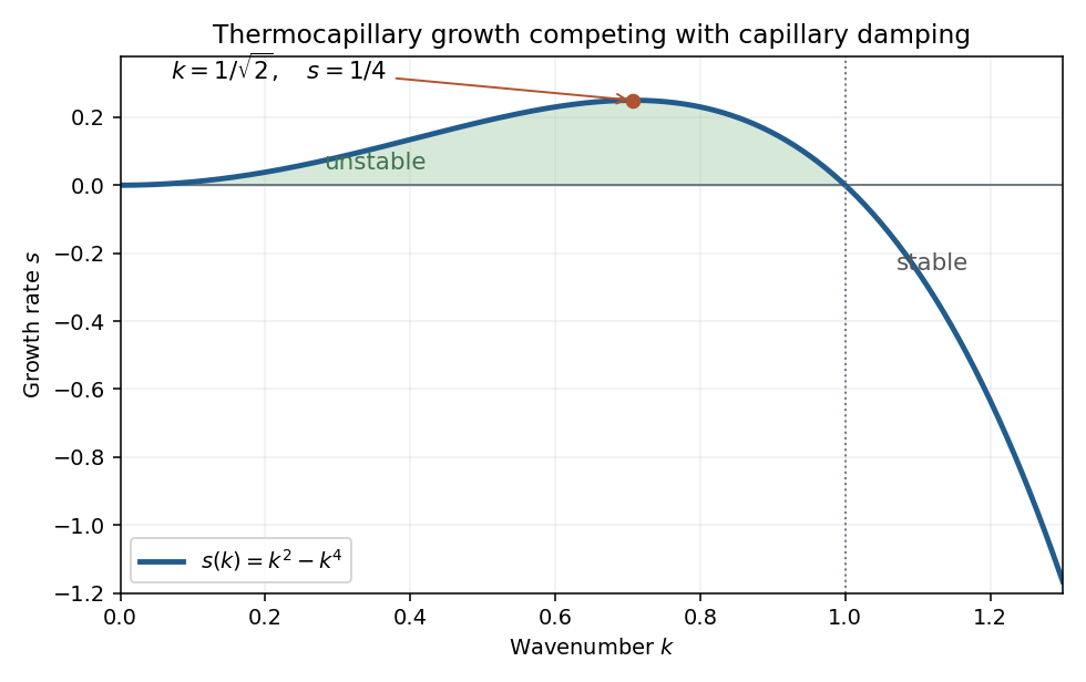
The capillary term smooths the film: a crest has negative curvature and higher liquid pressure, causing flow away from it. The thermal term has the opposite effect. A thicker region has a colder surface and therefore higher surface tension; Marangoni stress pulls surface fluid toward that region, reinforcing the thickness disturbance. These mechanisms give fourth-order damping and second-order growth respectively.

Use $H=h/\hat{h}$, $X=ϵx/\hat{h}$, and $\tau =t/\hat{t}$. The two dimensionless flux-divergence coefficients are $B{ϵ}^2\hat{t}/(2\mu )$ and ${\gamma }_0{ϵ}^4\hat{t}/(3\mu \hat{h})$. Setting both equal to one gives the balanced scales for a thermocapillary film:These choices yield $H_{\tau }+(H^2{H}_X{)}_X+(H^3{H}_{XXX}{)}_X=0$. The predicted $ϵ$ must be small for the assumed long-wave approximation.

Linearize about $H=1$ using a normal mode of amplitude $\delta$. The resulting equation is $s-k^2+k^4=0$, so the dispersion relation isModes with $0<|k|<1$ grow, while $|k|>1$ modes decay. Differentiating $s$ gives the most unstable wavenumbersThe physical fastest wavenumber is $ϵ/(\sqrt{2}\hat{h})$.

For a positive steady film with zero volume flux, $H^2{H}_X+H^3{H}_{XXX}=0$. Divide by $H^3$ and integrate once:Choosing the thickness scale so that $H=1$ when $H_{XX}=0$ sets $C=0$. Multiply $H_{XX}=-\ln H$ by $H_X$ and integrate to obtain the zero-flux thermocapillary film profiles relationThus the stated potential is $V(H)=H(\ln H-1)$ and the integration constant $E$ is the corresponding first integral.

In a slender symmetric viscous sheet, the two broad faces have zero tangential traction. A cross-thickness variation of $w$ on the thickness scale would produce leading shear $\mu w_x$, whereas $\mu u_z$ is smaller by the square of the aspect ratio. The leading transverse momentum balance and the shear-free conditions therefore give $w_x=0$: write $w=w(z,t)$.

Incompressibility gives $u_x=-w_z$. Symmetry about $x=0$ sets the integration constant to zero, soThe normal traction on either nearly vertical face matches the ambient hydrostatic pressure, giving ${\sigma }_{xx}=-p_a$ to leading order. The Newtonian fluid stress tensor then yieldsThe factor four is the planar extensional resistance, as in the planar viscous-sheet stretching equations, rather than the factor three for uniaxial extension with two contracting transverse directions.

The following slice diagram shows all axial-force contributions per unit $y$-width; the end arrows indicate positive tensile stress and reverse if that signed stress is negative.

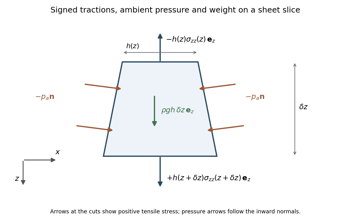
The two end tractions have net $z$-component ${\partial }_z(h{\sigma }_{zz})\delta z$. The normal pressure on the inclined side faces contributes $p_a{h}_z\delta z$, and gravitational acceleration gives the weight $\rho gh\delta z$. Hence force balance isSubstitute the stress expression and $p_a^{\prime }={\rho }_{a}g$:soKeeping the side-pressure component is essential: dropping it would retain an incorrect dependence on the arbitrary ambient pressure level. The remaining equation from conservation of mass isIt follows either by integrating incompressibility across the moving faces or directly from the face kinematic boundary condition.

When effective gravitational acceleration vanishes, $4\mu h{w}_z$ is independent of $z$. It equals the applied excess tensile force $F(t)$, with ambient pressure removed from the end loading. Along a material element labeled by its initial position $z_0$,Integration gives uniform material thinning under planar-sheet tension:A material interval conserves its area: $h(z,t)dz=h_0(z_0)d{z}_0$. ThusWith the specified fixed material origin, integrate the latter relation to obtainThese formulas hold while the material thickness remains positive.

For the quadratic initial profile, put $q=H-\Delta >0$. If $k\ne 0$, evaluating the integral at $z_0=L_0$ givesFor $k=0$ it instead givesFor a constant positive pulling force, $\Delta =Ft/(4\mu )$ first reaches the minimum initial thickness $H$ atBoth expressions for $L$ diverge there. Write $q=F(t^{\ast }-t)/(4\mu )$. If $k\ne 0$, the inverse tangent tends to $\pi /2$ and $\Delta \to H$, givingFor $k=0$,This is finite-time extension of a quadratically thickened sheet. With nonzero $k$, the dominant extension comes from the small material region $|z_0|=O(\sqrt{q/H}/|k|)$ near the thickness minimum, where the integrand is proportional to $1/(q+H{k}^2{z}_0^2)$. Its width shrinks like $\sqrt{q}$, giving an integrated divergence $q^{-1/2}$. The fixed ends are asymptotically far away in those local coordinates, so $A$ does not depend on $L_0$. For a uniform sheet the entire material interval has denominator $q$, giving the stronger $q^{-1}$ divergence and retaining its length in $A$. The singularity is a prediction of the ideal slender-sheet model as its minimum thickness tends to zero.