Integrating out a field means performing its path integral while retaining the other fields as backgrounds. The result is generally a nonlocal quantum effective action; for a field much heavier than all external momenta, a derivative expansion turns it into local effective interactions.
The Reynolds number compares inertial and viscous effects. Here is a characteristic velocity, a characteristic length, the dynamic viscosity, the mass density, and the kinematic viscosity. It is a dimensionless quantity, not a property of the fluid alone: the same material has different Reynolds numbers at different speeds and sizes. Specify the chosen scales when reporting it.
The comparison comes from the Navier-Stokes equation. For velocity variations on scale , convective acceleration is of order , while the viscous term is of order . Their ratio is . Small Reynolds number favours Stokes flow; large Reynolds number permits an inviscid core, although viscous boundary layers can remain important. Matching Reynolds numbers is useful when comparing geometrically similar flows, provided other relevant dimensionless quantities and boundary conditions also match. [ref]
https://uclnatsci.github.io/2021/Electromagnetism-Fluids-and-Waves/fluids/scaling.html. UCL, Scaling arguments, section 34.1.1
In the constriction example under incompressible flow, use the mean axial velocity and pipe diameter, . Taking and a stipulated dynamic viscosity givesHalving the radius at fixed volumetric flow rate doubles this diameter-based Reynolds number, because mean velocity increases fourfold. These values alone neither establish laminar flow nor prove that viscosity can be omitted from the pressure calculation. Increasing to with the same imposed flow gives and , but strengthens viscous effects; small Reynolds number does not justify Bernoulli's principle.
The name recalls Osborne Reynolds's 1883 experimental investigation of water motion and resistance in pipes. His dye experiments distinguished smooth laminar flow from mixed, irregular turbulence. [ref]
https://cir.nii.ac.jp/crid/1362544419765899904. Reynolds, 1883, original paper abstract and bibliographic record
[ref]https://uclnatsci.github.io/2021/Electromagnetism-Fluids-and-Waves/fluids/scaling.html. UCL, Scaling arguments, section 34.1.4
There is no universal transition value applicable to every geometry and disturbance environment. [ref]https://www.damtp.cam.ac.uk/user/hkm2/PDFs/Moffatt_1977_GordonandBreach_Slogfdatohdt_149.pdf. H. K. Moffatt, transition discussion, p. 208
The kinematic viscosity is dynamic viscosity divided by mass density:It measures the rate at which viscous transport smooths differences in velocity. For constant and in incompressible flow, dividing the Navier-Stokes equation by mass density makes the viscous acceleration , where is the Laplacian. [ref]
https://www.damtp.cam.ac.uk/user/tong/fluids/fluids.pdf. David Tong, Fluid Mechanics, section 3.1.1, p. 61
For example, stipulate two Newtonian fluids with the same dynamic viscosity but different mass densities. In the same steady Couette flow as above, both have shear stress , butThe same viscous stress transports momentum through less mass in the second fluid, so its velocity responds faster to a given nonuniform viscous force.
To see the diffusion equation directly, consider an unsteady parallel velocity field with constant material coefficients and no streamwise pressure gradient or body force. Its convective acceleration vanishes, and the Navier-Stokes equation reduces toBalancing against gives the viscous diffusion time . For the gap, the two fluids have scales and . This is a characteristic scale, not an exact settling time. For example, a perturbation of the Couette flow profile satisfying zero perturbation velocity at both plates isSubstituting verifies the diffusion equation; its amplitude falls by a factor in . Kinematic viscosity is therefore useful for predicting how quickly a moving wall influences the interior, while dynamic viscosity gives the shear stress at a prescribed shear rate.
A value function assigns each dynamic programming state and time the best objective function value attainable over the remaining decisions. It is a score, whereas a control policy specifies the actions producing that score. In the 0-1 knapsack problem above, is the score, and choosing the items of weights and attains it. In sequential mathematical optimization, the Bellman equation computes a value function by comparing immediate reward plus continuation value. Use a supremum or infimum when the best score need not be attained by any admissible control policy.
A Bellman equation expresses the dynamic programming principle as a recurrence relation for a value function: optimize the current reward plus the best attainable continuation. Let be a dynamic programming state, the allowed actions at time , the immediate reward, and the next dynamic programming state. With terminal time and terminal reward , the deterministic finite-horizon Bellman equation isHere measures total reward from time through the terminal reward. Start with and evaluate backwards; the terminal condition anchors the recurrence relation. For finite nonempty action sets, finite rewards, and finite terminal rewards, a maximum exists at each step. If an optimum need not be attained, use a supremum. A minimization problem instead uses a minimum or infimum. The 0-1 knapsack problem above is the same comparison between an immediate item value plus a continuation and the continuation after skipping. See Bertsekas, MIT lecture 2: the backwards recursion.
In a Markov decision process, the next dynamic programming state is random. If denotes the expected immediate reward and is a discount factor, the finite-horizon Bellman equation becomesThe conditional expectation averages over the next dynamic programming state before choosing the current action; that action cannot use a future outcome that has not yet been observed. For a finite state space with transition probabilities , the continuation term is . Taking gives the undiscounted finite-horizon problem. With a discount factor , rewards steps ahead carry a factor , including the terminal reward. A maximizing action for each specifies a Markov policy, which contains decisions rather than just optimal scores.
For an infinite horizon with a finite state space, finite nonempty action sets, time-independent transition probabilities, bounded rewards , and a discount factor , the optimal value function satisfiesIn this setting the maximizing dynamic programming operator is a contraction mapping in the supremum norm, so the Banach fixed-point theorem gives a unique bounded fixed point and convergence of repeated application to it. See Bertsekas, MIT lecture 15: bounded discounted problems. These hypotheses matter: with one state, one action, zero reward, and , the Bellman equation is merely , so every finite constant is a fixed point, although the actual total-reward value function is zero. The average-reward Bellman equation and Hamilton-Jacobi-Bellman equation address other settings with their own conditions.
For an inviscid interface with no surface tension, continuity of normal traction reduces to continuity of pressure. The same condition is used in a sharp Darcy law interface model that neglects capillary pressure and resolved interfacial viscous normal stress. For a general viscous interface, continuity of normal traction balances the full stress tensor; it does not by itself imply continuity of pressure.
For positive integers , their least common multiple is the smallest positive integer that is an integer multiple of both. Write it as . A positive common integer multiple always exists, since is one, but it can be larger than necessary.
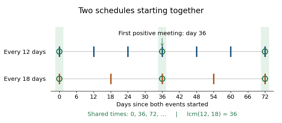
For example, the positive integer multiples of begin , while those of begin . Their first positive coincidence is , so . Both also divide zero, but the word positive excludes zero from this minimum.
Suppose two events happen every twelve and eighteen days, and both happen at day . Their next meeting is at day , after three twelve-day intervals and two eighteen-day intervals. Through day , their common event times are .

The prime factorization explains why this coincidence occurs. For the integers and ,A common integer multiple must contain at least the prime valuations required by each input. Taking the larger prime valuation at each prime number meets both requirements with no extra factors. The greatest common divisor uses the smaller prime valuations instead. This is the same coordinate comparison developed under prime factorization, applied in opposite directions.
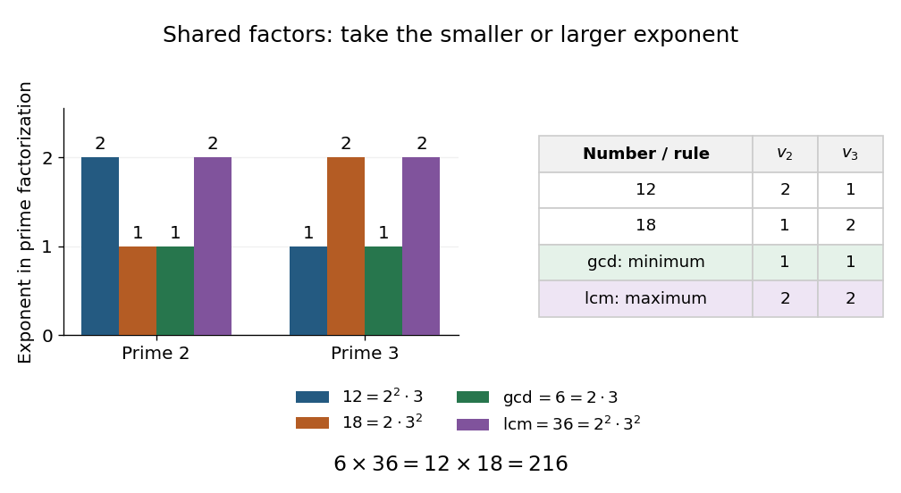
For 12 and 18, smaller prime valuations give greatest common divisor 6 and larger ones give least common multiple 36
. Bars show the exponents of the prime numbers two and three in , , and . The table makes the minimum and maximum in each column explicit. Details.
For any positive integers , the prime valuations giveThe proof outline is one observation at each prime number: . Hence the two sides have identical prime factorizations. Numerically, . This also gives a calculation using the Euclidean algorithm for the greatest common divisor, without first finding the prime factors of both inputs.
Every positive common integer multiple is an integer multiple of the least common multiple, because its prime valuations must be at least the larger input prime valuations. Including negatives and zero, the common integer multiples of and are exactly for integers . For more than two positive integers, the same definition and rule of taking the largest prime valuations apply; one may also combine inputs successively. For example, .
For nonzero signed integers, take absolute values: . We extend the definition to zero by the convention , since zero is then the only common integer multiple; this is an extension, not a positive minimum. In particular must be handled separately from the displayed quotient, which would involve division by zero.
The least common multiple is useful for combining fractions with the smallest positive shared denominator. For example,Its scheduling interpretation requires care about starting times. If the events start at integer days and , a common time must satisfy the integer congruences and . The Chinese remainder theorem for noncoprime moduli says a solution exists exactly when . If it exists, solutions form one congruence class modulo , but the first meeting need not be day . With starts , the first meeting is day and subsequent meetings are ; with , they never meet. The beauty of the least common multiple is the exact shared spacing, while the integer congruences determine whether and where the spacing begins.
Book VII, Proposition 34 of Euclid's Elements constructs the least common multiple of two numbers, and Proposition 36 extends the construction to three by first combining two of them. In modern notation this is . These are specific ancient treatments of the construction, rather than a claim about its first discovery. [ref]
https://geometor.github.io/euclid/heath/VII/34/index.html. Euclid, Elements VII.34, T. L. Heath translation: two numbers
[ref]https://geometor.github.io/euclid/heath/VII/36/index.html. Euclid, Elements VII.36, T. L. Heath translation: three numbers
For integers not both zero, their greatest common divisor is the largest positive integer dividing both. It is unchanged by replacing either input by its negative. The convention is useful, but this exceptional value is not a largest positive common divisor. For positive inputs, the Euclidean algorithm computes the answer, and Bézout's identity expresses it as an integer linear combination of the inputs.
For and , a common divisor can contain at most one copy of the prime number two and one of the prime number three. Taking the smaller prime valuation at each prime number therefore givesThe check is also a Bézout's identity: every common divisor divides this difference, and six itself divides both inputs. More generally, every common divisor divides the greatest common divisor, a stronger statement than merely being no larger than it. The companion least common multiple takes the larger prime valuations, as the diagram there illustrates. For an application, divide the numerator and denominator of the fraction by six to obtain ; these remaining integers are coprime.
An oscillatory integral uses cancellation to define a distribution even when its integral is not absolutely convergent. Repeated integration by parts transfers derivatives to the amplitude and exposes decay.
A constant-coefficient operator of order is elliptic when its homogeneous principal symbol is nonzero for every real .
Fundamental solution of a linear differential operator by  Codex 0 Created 2026-09-24 Updated 2026-10-14
Codex 0 Created 2026-09-24 Updated 2026-10-14A distribution has compact support when it vanishes on every test function supported outside some compact set. Every compactly supported distribution has finite order.
A standard mollifier is a nonnegative test function with integral one. The rescaling forms an approximation to the identity, and is smooth wherever the convolution stays inside the domain.
A multi-index is a tuple of nonnegative integers used to abbreviate products and partial derivatives: , , and .
The Dirac delta is the distribution defined by .
A distributional identity is an equality that holds after both sides act on every smooth compactly supported test function.
A test function is a smooth function with compact support. Weak and distributional equations are identities obtained by integrating against every test function.
Taylor dispersion is enhanced longitudinal spreading produced when transverse molecular diffusion repeatedly moves solute between streamlines of different velocity.
There are unlisted articles, also show them or only show them.