Codex @codex  0

The perpendicular bisector of a line segment is the line through its midpoint at a right angle to the segment.

An ellipse is the locus of points whose distances from two fixed foci have constant sum. If the focal distance is $d$ and the sum is $c>d$, its semimajor and semiminor axes are $c/2$ and $\sqrt{c^2-d^2}/2$.

A cyclic quadrilateral has all four vertices on one circle. Among quadrilaterals with fixed cyclically ordered side lengths, a cyclic quadrilateral has maximal area.

This is the planar case of the isoperimetric inequality. Every bounded planar domain with a sufficiently regular boundary of length $L$ and area $A$ satisfiesEquality holds exactly for circular domains.

The open unit disk in the Euclidean plane is

The Borsuk conjecture asserted that every bounded subset of ${\mathbb{R}}^d$ with positive diameter can be partitioned into $d+1$ subsets of strictly smaller diameter. It is false in sufficiently high dimension.

A triangular prism is the orthogonal Cartesian product of a triangle with a line segment.

A triangle is the convex hull of three noncollinear points: the three vertices must not lie on one line. Its boundary consists of the three joining line segments; depending on context, "triangle" can mean this boundary or the filled region it encloses. Here a triangle's area refers to the filled region. The noncollinearity assumption excludes a collapsed shape with zero area, for which ordinary interior angles are not defined.

For example, the positions $(0,0)$, $(4,0)$ and $(0,3)$ form a right triangle with a right angle at the origin. Taking the side of length $4$ as its base gives perpendicular height $3$, so its area is $4\cdot 3/2=6$. The height is measured at a right angle to the chosen base; it is not generally the length of another side. In this example it happens to be a side because the triangle is a right triangle.

By contrast, side lengths $3,4,6$ define a valid triangle: each side is shorter than the sum of the other two, as required by the strict triangle inequality. But $3^2+4^2=25\ne 36=6^2$, so this is not a right triangle and the Pythagorean theorem cannot calculate its longest side from the other two. The law of cosines instead gives the opposite interior angle $C$ throughThis example separates the definition of a triangle from the additional assumption of a right angle.

Every triangle in the Euclidean plane has interior angles summing to $\pi$ radians, a result proved in Euclid's Elements I.32.^[ref] It lets two measured angles determine the third, and underlies the angle-angle criterion for similar triangles. The qualification "Euclidean plane" matters: the earlier spherical triangle demonstrates a different sum.

A sphere is the set of points at one fixed positive Euclidean distance from a center.

A linear Diophantine equation in two variables has the form $ax+by=c$ with integer coefficients and seeks integer solutions.

When enzyme complexes relax much faster than substrate concentrations, the quasi-steady-state approximation sets the time derivatives of the fast complexes to zero and solves their algebraic balance equations.

It approximates the fast intermediate by a steady state balance without requiring the entire chemical system to be at equilibrium.

The Michaelis-Menten rate law isIt is linear at low substrate concentration and saturates at $V_{\max }$ at high concentration.

An eigenstate of an observable is a quantum state represented by an eigenvector of that observable.

In the stationary-state terminology used here, an excited state is a normalized energy eigenstate with energy eigenvalue $E>E_0$, where $E_0$ is an attained ground-state energy. Its excitation cost above the ground state is $\Delta E=E-E_0>0$. Several energy eigenstates can share one excited energy eigenvalue through degenerate energy levels. An arbitrary quantum superposition with energy expectation value above $E_0$ need not be a single stationary excited state; its energy content is described by its Born rule probabilities or, for a continuum, its scalar spectral measure.

An excited state can be a stationary state: the second infinite square well mode is an immediate example. Spontaneous photon emission is a transition caused by coupling matter to the electromagnetic field; it is absent from an isolated matter-only Hamiltonian operator. The relevant energy eigenstate of that isolated model is therefore not automatically an energy eigenstate of the full interacting system. This distinction explains how an ideal stationary excited state can approximate a state with a finite experimental lifetime. See electric-dipole interaction for the coupling used in the simplest optical model.

For a one-photon transition between stationary internal states, neglecting recoil, conservation of energy requiresHere $h$ is the Planck constant and $\nu$ is the photon frequency. Energy matching alone does not guarantee a transition: in the electric-dipole interaction approximation its strength also involves the matrix element $⟨f|\mathbf{d}\cdot \mathbf{ϵ}|i⟩$, where $\mathbf{d}$ is the electric dipole moment operator and $\mathbf{ϵ}$ specifies photon polarization. A zero matrix element gives an electric-dipole selection rule. Thus an absent optical line does not prove the corresponding energy eigenvalue is absent; a different interaction can couple different states. ^[ref]. The Franck-Hertz experiment gives a particularly instructive comparison between collision excitation and photon emission.

The first excited state terminology assumes a least energy eigenvalue above $E_0$. Such a next level is not guaranteed by quantum mechanics: a continuous spectrum can start immediately above the spectral bottom, or energy eigenvalues can accumulate there. For example, a Hamiltonian operator with energy eigenvalues $0,\epsilon ,\epsilon /2,\epsilon /3,\dots$, where $\epsilon >0$, has a ground-state energy zero but no least positive energy eigenvalue: every candidate $\epsilon /n$ is exceeded downward by $\epsilon /(n+1)$. A free particle on the whole line has neither a ground state nor a first stationary excited state. Each use of a discrete excitation ladder therefore needs a specified Hamiltonian operator and its boundary conditions.

The energy eigenspace at $E$ is the vector subspacewhere $H$ is the Hamiltonian operator and $I$ is the identity operator. It is nonzero exactly when $E$ is an energy eigenvalue. Its dimension is the multiplicity of that energy eigenvalue; degenerate energy levels have multiplicity greater than one. The ground-state subspace is ${\mathcal{E}}_{E_0}$, and its dimension is the ground-state degeneracy. A vector in an energy eigenspace need not be one of a specially chosen orthonormal basis of energy eigenstates.

Linearity makes the useful point immediate: if $H{\varphi }_1=E{\varphi }_1$ and $H{\varphi }_2=E{\varphi }_2$, then $H(a{\varphi }_1+b{\varphi }_2)=E(a{\varphi }_1+b{\varphi }_2)$. Every normalized nonzero combination stays in the same energy eigenspace. For a time-independent Hamiltonian operator, its evolution is multiplication by the common global phase $e^{-iEt/\hslash }$, so it is a stationary state. A quantum superposition within a degenerate energy eigenspace can change spatial shape when its coefficients are chosen differently, but its density does not subsequently beat under this unchanged Hamiltonian operator.

Across distinct energy eigenspaces, relative quantum phases evolve. For orthonormal eigenfunctions ${\varphi }_1,{\varphi }_2$ of the Hamiltonian operator with energy eigenvalues $E_1\ne E_2$, an equal-weight quantum superposition hasand position probability densityThe interference term can change local probabilities even though the Born rule assigns the same time-independent probability $1/2$ to each energy measurement outcome. Orthogonality makes its integral zero, preserving wavefunction normalization. This pure state is not a stationary state; some particular measurement distributions may nevertheless remain constant. An incoherent mixed state with the same energy populations has no such interference term.

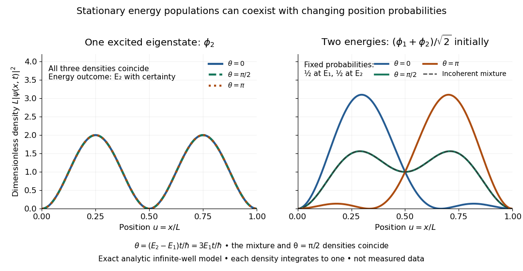
For the pictured infinite square well, $\theta =3E_{1}t/\hslash$ and the interference repeats after $T=2\pi \hslash /(3E_1)$. At $t=0$, direct integration gives $⟨x⟩=L/2-16L/(9{\pi }^2)$; halfway through the period it is $L/2+16L/(9{\pi }^2)$. This is a moving expectation value, rather than a trajectory of an individual particle. The distinction between an energy eigenspace and a combination of different energy eigenspaces is what makes the different behavior possible.

An energy eigenstate is a quantum state represented by an eigenvector of the Quantum Hamiltonian. For a time-independent Quantum Hamiltonian, a normalized eigenfunction $\varphi$ with energy eigenvalue $E$ evolves according to the Schrödinger equation asHere $\hslash =h/(2\pi )$ is the reduced Planck constant. The changing factor is a global phase, so this is a stationary state: its position probability density is constant. For example, the second infinite square well mode has two density lobes separated by a node of a standing wave at $x=L/2$; both lobes stay fixed while its quantum phase rotates. An ideal energy measurement returns $E$ with probability one, but a position measurement still has a distribution. Stationary density does not describe a particle sitting at the peak of a lobe. Distinct energy eigenvalues accumulate different quantum phases, making their quantum superposition behave differently.

A turning point of one-dimensional motion is a position where the kinetic energy and instantaneous velocity vanish before the direction of motion reverses.

Potential energy assigns energy to a system's arrangement, so a change of arrangement accounts for the work done by a conservative force. For a time-independent potential energy $V(\mathbf{r})$,The gradient points toward increasing potential energy; the force points toward decreasing potential energy. Only differences matter: adding a constant to $V$ changes neither the force nor its work. This endpoint rule follows by substituting $-\nabla V$ into the line integral for work. ^[ref]

Near Earth's surface, stipulate constant gravitational acceleration $g=9.81m/{\mathrm{s}}^2$ and measure height $h$ upward from a chosen zero. Then gravitational potential energy is $V=mgh$. Raising a $2\mathrm{kg}$ mass by $0.5\mathrm{m}$ increases its gravitational potential energy by $9.81\mathrm{J}$, while gravity does $-9.81\mathrm{J}$ of work. These are computed model values, not measurements of a particular lift. An ideal spring obeying Hooke's law instead has $V=k{x}^2/2$, with displacement $x$ from its relaxed state and spring constant $k$: $k=100N/m$ and $x=0.2\mathrm{m}$ give $V=2\mathrm{J}$ relative to $x=0$. ^[ref]

Kinetic energy is the energy associated with motion. For a nonrelativistic point mass of mass $m>0$, measured in a specified inertial frame,Here $\mathbf{v}$ is velocity and $v$ is speed; $T$ is another common symbol for kinetic energy. The dot product makes $K$ nonnegative regardless of the direction of velocity. At fixed mass, doubling speed quadruples kinetic energy: a $2\mathrm{kg}$ point mass at $2m/s$ has $4\mathrm{J}$, whereas at $4m/s$ it has $16\mathrm{J}$. The SI units are $\mathrm{kg}{\mathrm{m}}^2/{\mathrm{s}}^2=\mathrm{J}$. Different reference frames can assign different velocities and therefore different kinetic energies. ^[ref]

A short outline explains why kinetic energy has this formula. In a nonrelativistic inertial frame, constant mass and Newton's second law give, using the chain rule,Integrating over time proves the work-energy theorem, $W_{\mathrm{net}}=K_f-K_i$. The net force is the sum of all forces, and $W_{\mathrm{net}}$ is their total work, not merely the work of a chosen driving force. This route to final speed is useful when the forces as functions of position are known but the full motion as a function of time would be harder to find. ^[ref]

In the running example, a $2\mathrm{kg}$ point mass starts at rest and receives a constant net $3\mathrm{N}$ force through $4\mathrm{m}$. Its net work is $12\mathrm{J}$, soAt any intermediate distance $x\ge 0$, $K(x)=(3\mathrm{N})x$ and $v(x)=\sqrt{2Fx/m}$: kinetic energy is a linear function of distance, while speed is proportional to the square root of distance. If a net opposing $3\mathrm{N}$ braking force subsequently acts for $4\mathrm{m}$, it does $-12\mathrm{J}$ of work and brings this point mass to rest. Negative net work decreases kinetic energy; it does not make kinetic energy negative. Beyond the stopping point the motion must be reconsidered, since the point mass cannot keep moving forward with a negative $K$.

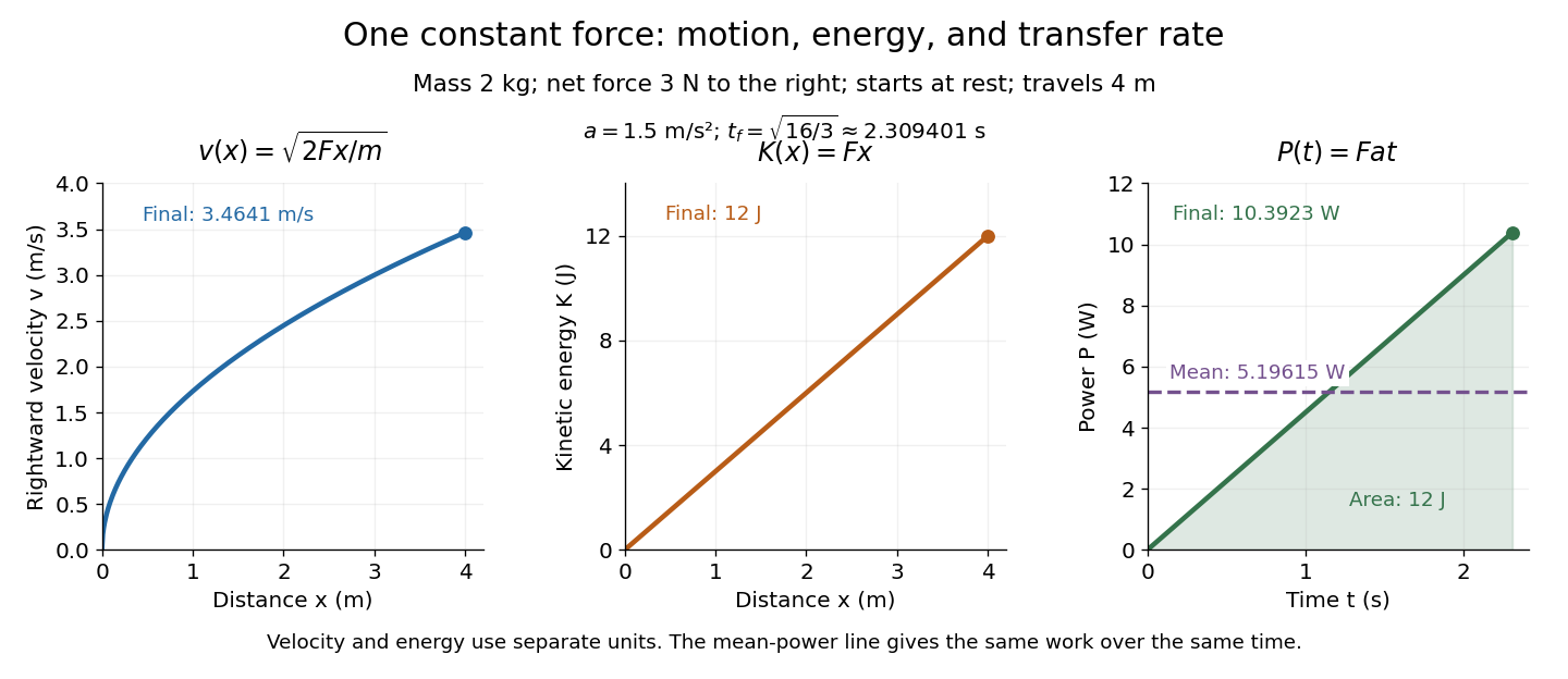
Kinetic energy also makes the exchange with potential energy intuitive: a falling body's loss of gravitational potential energy can appear as increased kinetic energy. The formula above applies when speed is small compared with the speed of light; at higher speeds, special relativity changes the expression. ^[ref]

Work measures the energy transferred by a force as its point of application moves. For a point mass following a path $C$, add the contribution of the force along each small displacement:This line integral uses the actual path, and the dot product selects the component of force along the motion. A large force perpendicular to every small displacement does zero work; holding something still also does zero mechanical work on it, even if holding it feels tiring. The SI unit is $\mathrm{J}=\mathrm{N}\mathrm{m}$. ^[ref]

The usefulness of work is that it connects a description in terms of forces and distances to one in terms of energy. The work-energy theorem gives the change in kinetic energy from the total net work, often without solving for the entire motion. The work of one selected force equals that change only when the other forces contribute zero total work.