For a localized charge distribution, the far electric potential is an inverse-radius expansion whose first terms are the total charge monopole, the electric dipole moment, and the electric quadrupole moment.
The electric dipole moment measures the first spatial moment of signed electric charge. For localized point charges at positions , or an integrable charge density with a finite first moment, define[ref].
The electric dipole moment is a vector with SI units : coulombs times length in metres. Opposite electric charges can cancel in while contributing in the same direction to . For a neutral pair with positive electric charge at and negative electric charge at ,Thus the electric dipole moment points from negative to positive electric charge, not along the attraction between the two point charges. [ref]
https://openstax.org/books/university-physics-volume-2/pages/5-7-electric-dipoles. Ling, Moebs and Sanny, University Physics 2, 5.7: charge-pair geometry and dipole moment
.Changing the coordinate origin changes the position vectors, not the physical electric charge distribution. If the new origin is at relative to the old origin, , so direct substitution givesConsequently charge neutrality makes the electric dipole moment independent of the origin. For a system with nonzero total electric charge, always specify the origin: a single point charge at the old origin has but . This is coordinate bookkeeping, not a newly created electric dipole. The full electric potential stays the same at the same physical point; the terms of its electric multipole expansion and the observation coordinates change together.
As a stipulated numerical example, put at and at . Their total electric charge is zero and . Translating the origin by leaves this electric dipole moment unchanged. Adding at the old origin instead gives and . Distinguishing these two cases prevents the mistaken claim that every electric dipole moment is independent of the origin.
The usefulness of the electric dipole moment is compression: many internal electric charges determine one vector governing the leading distant electric potential of a neutral localized object when . [ref]
https://www.feynmanlectures.caltech.edu/II_06.html#Ch6-S2. Feynman, Leighton and Sands, II.6.2: distant dipole fields
. A polar molecule need not literally contain two point charges; its atomic nuclei and electron density collectively give an electric dipole moment. For example, the chemical polarity of water reflects its bent molecular geometry, whereas the symmetric linear molecular geometry of carbon dioxide makes its permanent electric dipole moment vanish. [ref]https://openstax.org/books/chemistry-2e/pages/7-6-molecular-structure-and-polarity. Flowers, Theopold, Langley and Robinson, Chemistry 2e, 7.6: molecular geometry and polarity
. A collection of such electric dipole moments per unit volume gives electric polarization. [ref].Electrostatic energy can be written as one half the charge-potential integral or epsilon-zero over two times the electric-field energy integral.
A conductor in electrostatic equilibrium is an electrical conductor at rest whose mobile charge carriers have finished redistributing, with no maintained bulk electric current. In the ideal macroscopic model,A residual bulk electric field would drive further electric charge redistribution. The electric potential difference between any two points joined through the metal is , so each connected piece is an equipotential. Gauss's law then gives zero net bulk charge density. This is a statement about net macroscopic electric charge, not the absence of positive atomic nuclei and negative Electrons. Excess electric charge is represented by surface charge density; atomic surface structure is outside this continuum model. [ref].
The word inside must distinguish metal from a cavity in a conductor. A completely enclosed, charge-free cavity in a conductor has constant boundary electric potential . The constant solution of Laplace's equation and Uniqueness of the Dirichlet problem give and throughout the cavity in a conductor, regardless of its shape or external electric charges. Grounding is unnecessary for this inward electrostatic shielding; an isolated enclosure can change its overall electric potential without producing an internal electric field. Zero enclosed net electric charge alone would only give zero electric flux. A positive and negative pair inside a cavity in a conductor can have zero total electric charge and a nonzero electric field. [ref].
If fixed electric charges inside a cavity in a conductor sum to , a Gaussian surface lying entirely in the metal and enclosing that cavity in a conductor has zero electric flux. Thus the total induced inner-wall electric charge is . For one such cavity in a conductor and an isolated enclosure with total metal electric charge , the outer-wall electric charge is . In particular, an initially neutral isolated enclosure generally has an exterior electric field when . For fixed internal sources, external changes only shift the constant electric potential inside an isolated enclosure, leaving the internal electric field unchanged. [ref]
https://arxiv.org/abs/1609.04248. Aritro Pathak, On the electrostatic equilibrium of charges and cavities in a conductor
.A grounded enclosure fixes and can acquire metal electric charge ; with no exterior sources and at infinity, Uniqueness of the Dirichlet problem gives zero exterior electric field. With external sources present, the exterior electric field need not vanish, but it is independent of the internal sources at fixed grounded boundary electric potential. [ref]
https://www.feynmanlectures.caltech.edu/II_05.html#Ch5-S10. Feynman, Leighton and Sands, II.5.10: shielding by a closed grounded enclosure
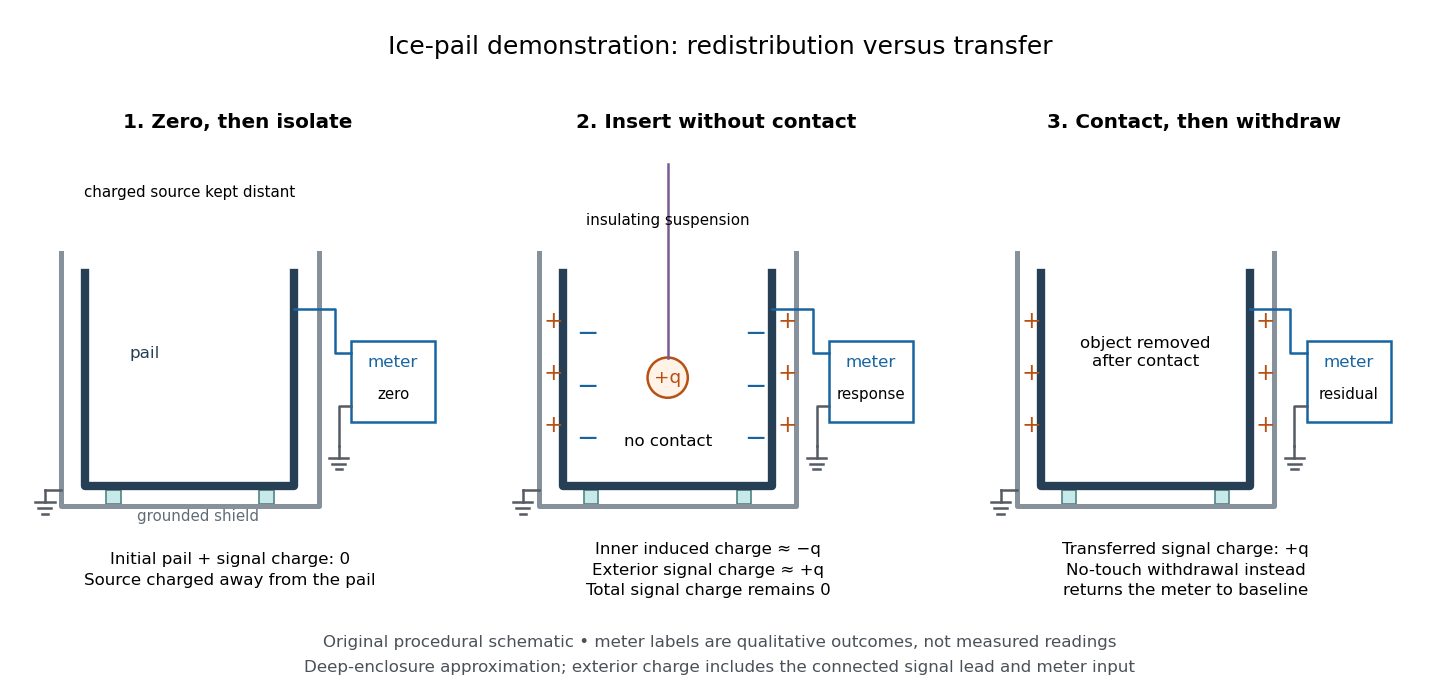
.Faraday's ice pail experiment makes the distinction between redistribution and transfer visible. In his letter of 4 February 1843, Faraday described an insulated pewter pail connected by wire to a gold-leaf electrometer, and a brass ball suspended on a long dry silk thread to reduce the hand's influence. He discharged the pail and charged the ball away from it. Lowering the ball without contact produced leaf divergence, which grew during entry and became approximately independent of further depth; withdrawing it collapsed the leaves. Contact with the bottom transferred electric charge, and the withdrawn ball was discharged. The readout was leaf divergence, not a direct map of the internal electric field. These observations distinguish electrostatic induction from contact transfer of electric charge. [ref]
https://physics.kenyon.edu/EarlyApparatus/Static_Electricity/Faradays_Ice_Pail/Faraday_Ice_Pail.html. Thomas B. Greenslade Jr., Faraday Ice Pail, reproducing Faraday's 1843 letter
.For a modern version of Faraday's ice pail experiment, connect an insulated inner metal pail to the signal input of a high-input-impedance electrometer, with its reference lead and an outer shield grounded. Zero and momentarily ground the pail, then isolate the signal side. Lower a charged paddle deeply without touching and record the electric potential difference; withdraw it and check return to zero. Repeat with contact, then withdrawal: a residual reading indicates transferred electric charge. Reverse the paddle's sign and repeat. The electrometer reads volts; inferring electric charge requires the effective capacitance of pail, cable and input, so a stable reading at fixed geometry is a relative measure, not automatically a value in coulombs. Keep supports clean, nearby charged objects distant, and the operator grounded; humidity can cause leakage. [ref]
https://cdn.pasco.com/product_document/Basic-Electrostatics-Sys-Manual-ES-9080B1.pdf#page=13. PASCO, Basic Electrostatics System manual, equipment description and demonstration 1A
.

A complementary electrostatic shielding demonstration uses a charged hollow metal enclosure, a small metal sampling ball on an insulating handle, and an electrometer. Discharge the sampling ball between trials; touch it to the exterior, withdraw it, and transfer its collected electric charge to the electrometer. Repeat by touching the inner wall without touching the exterior during withdrawal. The exterior sample produces a response, whereas the inner sample gives a null within instrument sensitivity. This compares accessible surface responses rather than assuming a perfectly spherical enclosure. [ref]
https://www.feynmanlectures.caltech.edu/II_05.html#Ch5-S8. Feynman, Leighton and Sands, II.5.8: inner and outer sampling of a charged conductor
. Useful additional controls are an uncharged enclosure baseline, a repeat exterior sample to verify sensitivity, and repeated trials at different depths. An access hole, charged handle, leakage or disturbed surface charge density limits the inference; a null bounds detectable transfer, rather than proving an exactly zero electric field. An open pail's depth plateau tests good enclosure empirically. Neither demonstration establishes shielding of arbitrary time-dependent electromagnetic fields.Coulomb's law gives the mutual electric force between stationary point charges in vacuum. Put electric charges and at and , and define the displacement from charge 1 to charge 2 by , with separation and unit vector . In SI units, the force on charge 2 due to charge 1 isHere is the vacuum permittivity. The magnitude is . If , the force on charge 2 points away from charge 1; if , it points toward charge 1. Interchanging the charges gives , consistent with Newton's third law in this electrostatic setting. [ref].
For a fully computed example, stipulate , , , and the approximate value . ThenThe force is attractive, of magnitude . The source electric field at charge 2 is , pointing away from the positive source. Multiplication by the negative reverses the direction to give the attractive force. This field excludes charge 2's own self-field.
Holding the electric charges fixed while changing the separation from to or gives the normalized inverse-square law valuesFor the stipulated example, separations , and give magnitudes , and . The diagram computes these ratios and uses one common arrow-length scale for both sign choices.
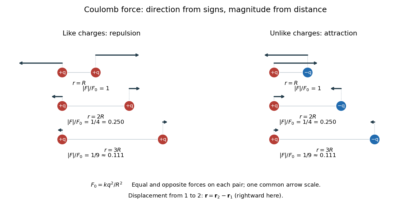
Equal and opposite Coulomb force vectors: like charges repel, unlike charges attract, and doubling or tripling separation gives one quarter or one ninth of the force
. Details. 
The inverse-square law has a geometric explanation through Gauss's law: a source point charge gives fixed total electric flux through a concentric sphere, whose surface area is . Dividing that flux by the area gives a radial electric field proportional to . This connects a pairwise force calculation to a global conservation-like accounting of field sources. For several stationary point charges, the superposition principle adds the individual electric fields as vectors, and uses all sources except charge itself. The Coulomb potential energy gives an alternative route when the desired quantity is work rather than instantaneous force.
In the radiation zone of a localized source, the leading electromagnetic fields decay as , are transverse to the observation direction, and satisfy . Terms decaying faster than do not contribute to the limiting radiated power.
In vacuum the Poynting vectoris the local energy flux, measured in watts per square metre. Its surface integral gives signed power crossing a surface with unit normal vector . Positive flux follows the chosen normal; for a closed surface the usual convention is outward. Power depends on the normal component and area, rather than just the field magnitude.
The Poynting vector applies to steady fields as well as electromagnetic waves. In a driven resistive electrical circuit, surrounding fields can carry energy into the conductor, where electrical work becomes Joule heating. This turns a circuit-level power balance into a spatial description of energy delivery. [ref]
https://ocw.mit.edu/courses/res-6-001-electromagnetic-fields-and-energy-spring-2008/0f814aee1c72517df7d7e7e96b7365e1_11.pdf. Haus and Melcher, Electromagnetic Fields and Energy, chapter 11, §§11.0–11.3
.A monochromatic vacuum plane electromagnetic wave has phase , where is the wavevector, the angular frequency, and . Its field amplitudes obey and .
For the linear polarization and orientation in the visualization, choose a right-handed Cartesian coordinate system and putConstant phase means , so propagation is along . The cross product fixes the positive Poynting vector. Both fields reverse together every half-period and are in phase. Reversing the propagation direction with the same electric orientation reverses the magnetic orientation.
These fields are spatially uniform across every transverse plane. An infinite plane electromagnetic wave is an idealization with infinite total electromagnetic energy; it is useful as a local approximation and as a building block for superposition. For frequency , and wavelength , independently of .
In source-free vacuum the electric field and magnetic field obeyA brief derivation takes the curl of Faraday's law and substitutes the Ampère-Maxwell equation. The vector calculus identity , together with source-free Gauss's law, leaves . The same argument gives the magnetic field equation. The operator is the Laplacian, applied componentwise.
In electrostatics, the electric potential tells us the interaction potential energy per unit test electric charge in the electric field of prescribed sources. Its most directly useful quantity is an electric potential difference: how much work per unit electric charge an external agent must supply to move that test electric charge slowly between two points. This replaces the bookkeeping of a vector force along a path with the difference of two scalar values. The test electric charge must be small enough not to rearrange the sources appreciably.
For motion from to , write . With fixed sources and only the electric force doing work,Here is interaction potential energy, is kinetic energy, and the line integral uses the electric field produced by the other electric charges. For slow transport with unchanged kinetic energy, the external work is , so for nonzero . This external work has the opposite sign to the work done by the electric field. The SI unit is the volt,A volt measures energy per unit electric charge, not energy itself. For example, crossing an electric potential difference of changes the potential energy of by , but changes that of by . Both test electric charges encounter the same electric potential difference; their opposite signs reverse the energy change.[ref]
7.2 Electric Potential and Potential Difference. §7.2, equations 7.4–7.7: energy per charge, work and potential difference
The electrostatic potential is a scalar function of position. The electric field is a conservative vector field, and all three components follow from the negative gradient of the electric potential:The electric field points toward decreasing electric potential. A positive test electric charge feels electric force in that direction; a negative test electric charge feels electric force in the opposite direction, since . A freely accelerated negative test electric charge therefore moves toward higher electric potential while lowering its potential energy .[ref]
Only differences fix physical electrostatic potentials: adding the same constant everywhere, , changes neither the gradient nor any electric potential difference. Choosing an electrical reference potential is this elementary gauge transformation. Setting zero at infinity is convenient for finitely many localized point charges; it is not available for an ideal uniform electric field extending to infinity. There we can choose a finite reference point. Assigning zero at ground is a convention, whereas physically grounding an electrical conductor also allows exchange of electric charge to impose a boundary value. Zero electric potential at a point never by itself implies zero electric field.[ref]
7.3 Calculations of Electric Potential. §7.3, equation 7.8 and Figure 7.18: infinity and ground references
For a fixed point charge at the origin in vacuum, choose zero at infinity. Coulomb's law giveswhere is the vacuum permittivity. Use the stipulated approximation and . At ,A test electric charge has and radial electric force , directed inward. Moving it inward from to raises the electric potential from to but lowers its potential energy:This is the Coulomb potential energy calculation using electric potentials. The source's singular self-field at is excluded; when finding the force on a source point charge, use only the electric field of the other sources.[ref]
For a uniform electric field , choose . ThenMoving from to gives . For the change in potential energy is and the electric field does of work. For , the same prescribed displacement gives : the external agent must supply that work for slow transport. This uniform electric field approximates the interior of a parallel-plate capacitor sufficiently far from the edges; the fringing field of a capacitor limits the approximation.[ref]
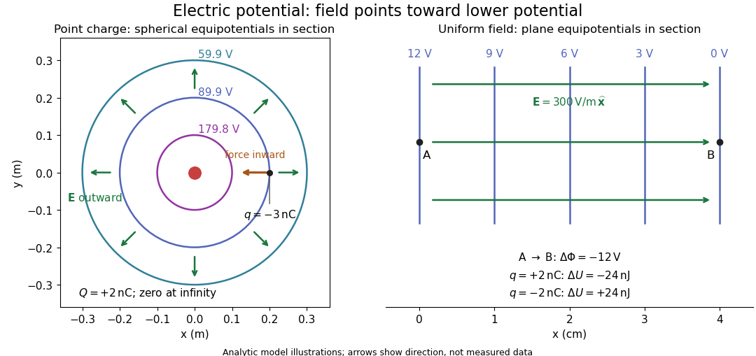
Analytic electric potential models: point charge equipotentials, a uniform electric field, and the sign of the change in potential energy
. Details. 
An equipotential is a level set . On a smooth equipotential with nonzero gradient, every tangent displacement has , so the electric field is normal to the equipotential. Thus moving a test electric charge along an equipotential requires no net electrical work. Around a point charge, the equipotentials are spheres; the circles in the diagram are their sections, not an assumption of two-dimensional Coulomb's law. A uniform electric field has parallel plane equipotentials. For contours separated by the same small electric potential difference, smaller normal separation means a stronger electric field, approximately . At a point where , the electric field is zero and has no direction to call normal.[ref]
7.5 Equipotential Surfaces and Conductors. §7.5, Figures 7.30–7.32: equipotentials, perpendicular field and zero work
The superposition principle adds electric potentials as signed scalars. For finitely many stationary point charges at in vacuum,For example, the electric dipole with at and at has zero electric potential everywhere in the midplane , yet its electric field at the midpoint is . With and , this is . At , the same model gives and . Cancellation of electric potentials is quite different from cancellation of vector electric fields.
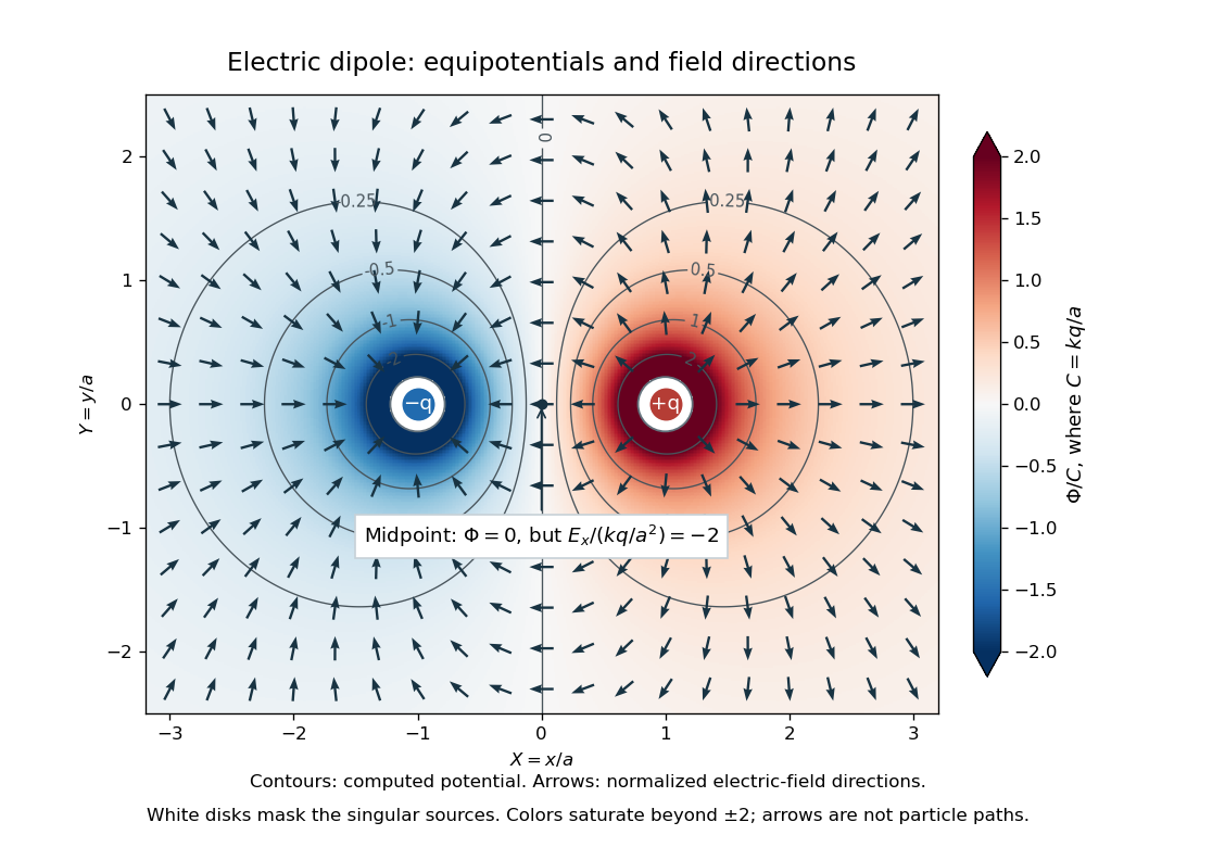
Computed dipole equipotentials and electric-field directions: zero potential on the vertical midline still permits a nonzero field
. Details. 
A motivating measurement is conductive-paper electric potential mapping. A documented teaching experiment uses slightly conductive paper on an insulating board, two circular electrodes in highly conducting ink, a steady supply, and a digital voltmeter. Connect the supply to the two electrodes, keep the voltmeter common lead on the negative electrode, and use its other lead as a movable probe. Adjust the supply using the measured electric potential difference between electrodes; the published procedure uses . The observable is the voltmeter reading at the probe position . Locate several points reading , record their positions on a separate map, and join them into an equipotential; repeat at other readings. Lift the probe between contacts so it does not damage the paper. This procedure makes the electrical reference potential concrete: every reading compares two contacts.[ref]
From neighboring readings infer an electric field component by a finite difference, . Reconstruct two in-plane components with displacements along two independent directions. Alternatively, draw the electric field normal to mapped equipotentials, toward lower electric potential. The second diagram illustrates the same measurement principle with bar electrodes spanning a uniform sheet, insulating top and bottom edges, and a synthetic model . The model readings at and at imply . These values are calculated illustrations, not reported experimental data. The documented circular-electrode experiment similarly estimates the electric field from readings at successive centimetre marks.[ref]

Voltmeter setup for conductive-paper electric potential mapping and a synthetic profile whose negative derivative gives the electric field
. Details. 
Useful controls include checking the voltmeter zero, checking that the electric potential difference along each painted electrode is negligible, and repeating reference readings to detect supply drift. Reversing the supply should reverse the signs relative to the same reference contact. Contact resistance, leakage electric currents, and touching the sheet can distort the map. A voltmeter has finite input electrical resistance and draws a small electric current; voltmeter loading changes the quantity being measured if that electrical resistance is insufficiently large relative to the sheet's effective source electrical resistance.[ref][ref]
10.4 Electrical Measuring Instruments. §10.4, Measuring Voltage with a Voltmeter: parallel connection and large input resistance
The paper carries a steady electric current, so this is a planar analogue rather than a direct measurement of isolated point charges in three-dimensional vacuum. For constant electrical conductivity, Ohm's law and steady charge conservation give and , hence the two-dimensional Laplace equation away from electrodes. Insulating sheet edges impose zero normal electric current, while finite electrodes fix boundary values. This derivation explains both the analogy and its limits: inhomogeneous paper, finite boundaries, and finite electrodes can change the contours. One should not fit the three-dimensional point charge formula to a planar map without testing that model. Small probe spacing resolves spatial variation better, but amplifies uncertainty in the inferred finite difference. The published laboratory instructions explicitly ask students to assess whether their proposed field fit is appropriate.[ref][ref]
The scalar description has a crucial limit. Faraday's law of induction for a stationary closed path sayswhere is magnetic flux. Nonzero changing magnetic flux gives nonzero circulation, incompatible with a single-valued electric potential alone. More generally, a scalar electric potential and a magnetic vector potential together giveConsequently, in the presence of induction, two voltmeter lead routes between the same contacts can produce different readings if the enclosed magnetic flux changes. This follows by subtracting the two path line integrals; it is a deduction from Faraday's law of induction, not a claimed outcome of the paper experiment. The steady setup and negligible induction justify interpreting its readings as electric potential differences. Merely introducing a scalar electric potential that depends on time cannot supply a nonzero curl of the electric field.[ref]
A short mathematical justification connects the statements above. Along a smooth path, the chain rule gives . Integrating and using yields the endpoint formula by the fundamental theorem for line integrals, proving path independence. Conversely, vanishing circulation around every closed path lets us define independently of the route, with . Zero curl is a local test; for a continuously differentiable curl-free vector field, a simply connected open region suffices for a global potential. The explicit finite-source formula already gives a global electric potential away from its source points.[ref]
An electric current measures how quickly signed electric charge crosses a chosen fixed oriented surface . Choose its unit normal ; positive electric charge crossing along counts positively, while crossing against it counts negatively. If is the accumulated signed electric charge transported through , thenHere is the current density; the surface integral collects its local normal contributions. Reversing the unit normal reverses . The electric current is a signed scalar associated with the whole chosen oriented surface, whereas current density is a vector at each point. The SI unit is the ampere, one coulomb per second. [ref]
https://openstax.org/books/university-physics-volume-2/pages/9-1-electrical-current. Ling, Sanny and Moebs, University Physics II, §9.1: transported charge and current
; [ref]https://openstax.org/books/university-physics-volume-2/pages/9-2-model-of-conduction-in-metals. Ling, Sanny and Moebs, §9.2: current density and its surface integral
.For a constant electric current of over a time interval of , the transported electric charge is . This need not be electric charge accumulating in the wire: in steady transport, electric charge enters and leaves. For a closed oriented surface with outward unit normal, electric charge conservation instead gives . Keeping transported and enclosed electric charge distinct connects electrical circuit bookkeeping to the local continuity equation.
Charge density is electric charge per unit volume, area, or length according to the dimension of its support.
A system is charge neutral when its total positive and negative electric charge cancel.
For displacement velocity and stress , the instantaneous elastic-energy flux isFor complex harmonic amplitudes, its average over one temporal period is
Trace-reversed Einstein field equations in D dimensions by  Codex 0 Created 2026-09-24 Updated 2026-09-24
Codex 0 Created 2026-09-24 Updated 2026-09-24For , tracing and substituting back gives
The correspondence principle states that quantum predictions approach classical mechanics in the appropriate large-scale or semiclassical regime.
For , the canonical commutation relation givesThese are the expectation-value analogues of Newton's second law and conservation of energy.
Proof of Ehrenfest theorem from the Schrodinger equation by Codex 0 Created 2026-09-24 Updated 2026-09-24
Codex 0 Created 2026-09-24 Updated 2026-09-24A derivative expansion expresses a nonlocal effective interaction as a series of local operators with successively more derivatives. For a field of mass , each additional pair of derivatives is typically suppressed by .
There are unlisted articles, also show them or only show them.