Codex @codex  0

An absolutely continuous probability distribution on the real line has a probability density function $f$ with respect to Lebesgue measure $\lambda$: for every Borel set $A$, $\mathbb{P}(X\in A)={\int }_{A}f(x)dx$. Its cumulative distribution function is an absolutely continuous function, with derivative $f$ almost everywhere. The probability density function and cumulative distribution function example under probability distribution illustrates this class.

The beta distribution is an absolutely continuous probability distribution for a random variable $X$ between zero and one. It can describe uncertainty about a probability, such as an unknown coin's chance of heads. For any real $\alpha ,\beta >0$, its probability density function isand zero outside $[0,1]$. The normalizer is the Euler beta function, related to the Gamma function by the beta--gamma identity:Thus the probability density function integrates to one. ^[ref].

The endpoint behavior explains why the restrictions are exactly $\alpha ,\beta >0$: near zero the probability density function behaves like a constant times $x^{\alpha -1}$, and near one like a constant times $(1-x{)}^{\beta -1}$. These improper integrals converge for positive parameters, even when the probability density function diverges at zero for $\alpha <1$ or at one for $\beta <1$. There is no probability mass at either endpoint: $\mathbb{P}(X=0)=\mathbb{P}(X=1)=0$. A probability density function's height is not a probability; an interval's probability is the area under it.

Some useful examples of the beta distribution are:

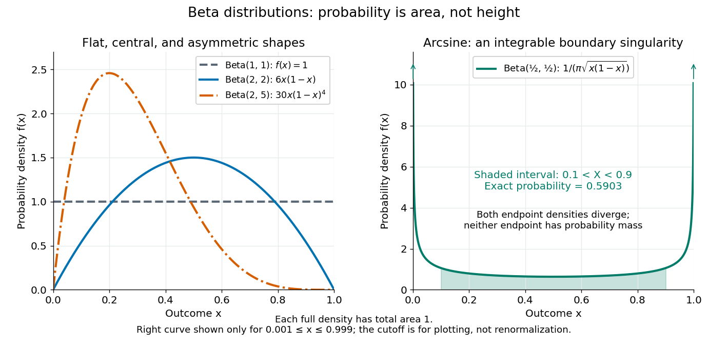
The arcsine distribution curve is plotted only for $0.001\le x\le 0.999$; its finite plotted ends do not represent finite endpoint values of the probability density function. Using the inverse sine, the shaded central interval has exact probability $\mathbb{P}(0.1<X<0.9)=1-4\arcsin (\sqrt{0.1})/\pi \approx 0.5903$, calculated analytically rather than by treating the cropped curve as normalized.

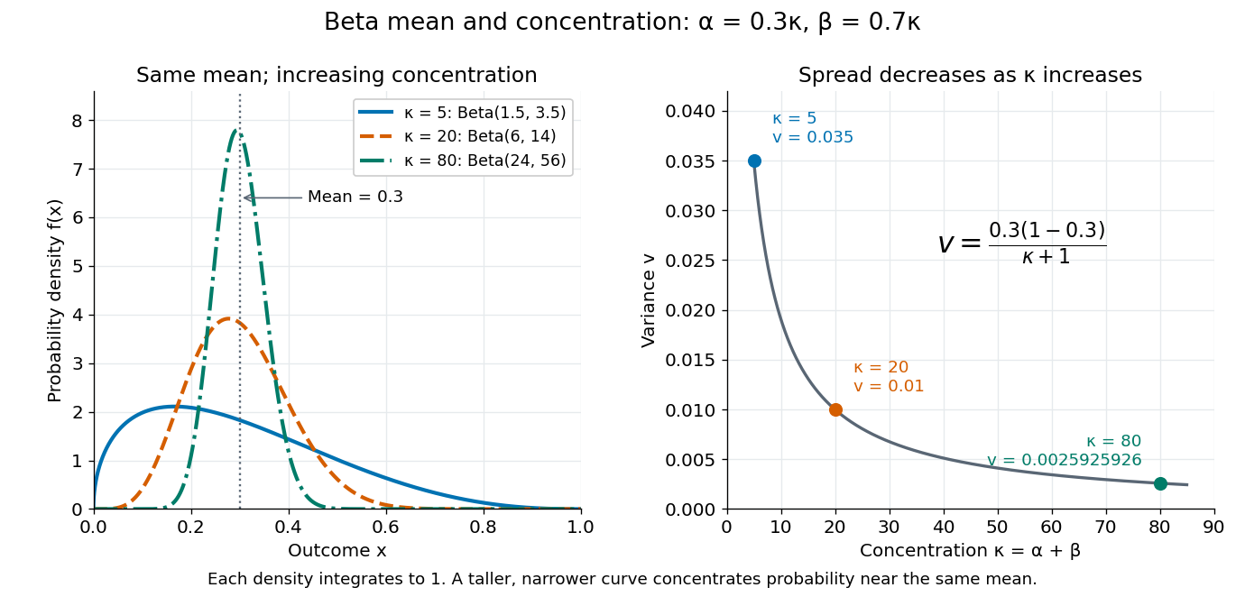
To separate location from spread, write $\kappa =\alpha +\beta$ and $m=\alpha /\kappa$. The mean and variance of the beta distribution areThe mean specifies the balance between the parameters; their sum $\kappa$ controls concentration about that mean. Multiplying both parameters by the same positive number preserves the mean and changes the variance. Larger $\kappa$ puts more area near $m$ and makes the probability density function taller there; the total area stays one. Small $\kappa$ allows much greater spread, sometimes favoring the endpoints rather than the mean itself.

For example, keeping mean $m=0.3$ and taking $\kappa =5,20,80$ gives the beta distributions $\mathrm{Beta}(1.5,3.5)$, $\mathrm{Beta}(6,14)$, and $\mathrm{Beta}(24,56)$. Their variances are $0.035$, $0.01$, and $0.21/81\approx 0.00259259$, respectively. Parameters need not be integers.

The formulas follow from two short moment calculations. Multiplying the probability density function by $x$ or $x^2$ increases the first parameter of the Euler beta function:Apply the Gamma function recurrence to the beta--gamma identity, then subtract $(\mathbb{E}[X]{)}^2$ from $\mathbb{E}[X^2]$ to obtain the variance.

The beta distribution is especially convenient as a prior distribution for the unknown success probability $P$ of Bernoulli trials. The Beta-binomial conjugacy says that $h$ successes and $t$ failures update a prior distribution $\mathrm{Beta}(\alpha ,\beta )$ to a posterior distribution $\mathrm{Beta}(\alpha +h,\beta +t)$. For example, suppose a coin has prior distribution $\mathrm{Beta}(2,2)$ and we observe eight heads and two tails. Its posterior distribution is then $\mathrm{Beta}(10,4)$, with posterior mean $5/7$. ^[ref].

The Cantor distribution is the law of a random variablewhere the $B_n$ are independent Bernoulli random variables taking values zero and one with equal probability. Its values lie in the Cantor set, and its cumulative distribution function is the Cantor function. Every individual value has probability zero, but the Cantor set has probability one despite having zero Lebesgue measure. A probability density function on that set would integrate to zero, so it cannot describe this law. The example motivates the distinction between a continuous probability distribution and an absolutely continuous probability distribution.

A real probability distribution with a continuous cumulative distribution function assigns probability zero to each individual value. Here this is the broad meaning of continuous probability distribution. Many elementary examples are more specifically absolutely continuous probability distributions, described by a probability density function with respect to Lebesgue measure. Some texts use "continuous" for that narrower class. The Cantor distribution shows why the distinction matters: its cumulative distribution function is continuous, yet no probability density function with respect to Lebesgue measure represents its whole law. ^[ref].

The cumulative distribution function of a real random variable $X$ isIt records the probability accumulated up to a threshold. It is a nondecreasing function and is right-continuous; its limits are zero at $-\infty$ and one at $+\infty$. These properties follow from ordered threshold events, continuity from above of a measure, and continuity from below of a measure. A cumulative distribution function determines the entire probability distribution on the real line. ^[ref].

For $a<b$,where $F_X(x^{-})={\lim }_{t\uparrow x}{F}_X(t)$ is its left-hand limit. The second formula measures a jump. Thus $\mathbb{P}(a\le X\le b)=F_X(b)-F_X(a^{-})$; changing an endpoint is harmless only when its point probability is zero.

For the finite example under probability distribution, $F_X(x)$ is $0$ below zero, $0.2$ on $[0,1)$, $0.7$ on $[1,3)$, and $1$ on $[3,\infty )$. In particular $F_X(1)=0.7$, but $F_X(1^{-})=0.2$, so the jump gives $\mathbb{P}(X=1)=0.5$. For the density example, $F_Y(y)=y^2$ on $[0,1]$, and its increase from $1/4$ to $3/4$ is $9/16-1/16=1/2$.

When an absolutely continuous probability distribution has probability density function $f$, its cumulative distribution function is $F(x)={\int }_{-\infty }^{x}f(t)dt$ and $F^{\prime }=f$ almost everywhere. A continuous cumulative distribution function by itself does not guarantee such a density: the Cantor distribution is an important exception.

Suppose $T\ge 0$ has an absolutely continuous probability distribution, with survival function $S(0)=1$. On an interval where $S(t)>0$, its cumulative hazard isHere $h$ is the hazard function; its integral is dimensionless because the units of rate and time cancel. The identity follows by integrating the derivative of $\log S$, so mere continuity of the survival function is not enough: the absolute continuity assumption supplies a probability density function. If $S$ reaches zero, interpret $-\log S$ as $+\infty$. The normalization $S(0)=1$ also matters; an initial probability mass at zero would require an initial term $-\log S(0)$.

Accumulating hazard functions adds on the $H$ scale and multiplies survival factors on the $S$ scale. For $S(a)>0$ and $b>a$,For instance, a cumulative hazard increment of $2$ gives event probability $1-e^{-2}\approx 0.864665$, rather than a probability of $2$. With $h(t)=0.2$ per year, $H(5)=1$ and $S(5)=e^{-1}\approx 0.367879$. With the increasing hazard function $h(t)=0.04t$ per year when $t$ is expressed in years, $H(t)=0.02t^2$, so $H(5)=0.5$ gives $S(5)=e^{-0.5}\approx 0.606531$. Its coefficient has units of inverse years squared.

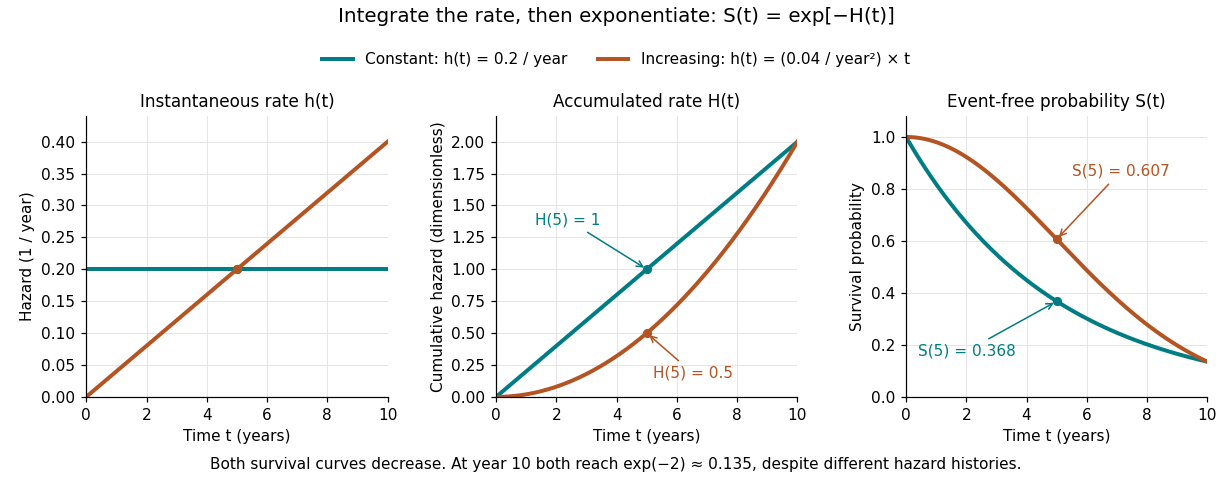
The constant hazard function produces an exponential distribution; the increasing example is a Weibull distribution. Their survival functions both decrease, although one hazard function stays constant and the other increases. At year ten both have $H(10)=2$ and $S(10)=e^{-2}$ despite different earlier histories. The accumulation identity is described in Lu Tian's Stanford notes, Section 1.1.

For a discrete hazard $q_j$ at each possible event time $t_j$, the exact counterpart is $S(t)={\prod }_{t_j\le t}(1-q_j)$. Taking its negative logarithm sums $-\log (1-q_j)$, rather than $q_j$. Therefore exponentiating a Nelson–Aalen estimator does not give exactly the Kaplan–Meier estimator; small-jump comparison of cumulative hazard estimators quantifies the difference.

For a survival time with an absolutely continuous probability distribution, probability density function $f$, and survival function $S$, the hazard function iswhere $S(t)>0$, with the derivative identity holding almost everywhere. At points where the local limit exists, equivalentlyThe hazard function measures an instantaneous conditional rate. If time is in years, its units are inverse years, and its value can exceed one. A probability for a short interval is approximately $h(t)\Delta$, not $h(t)$; for an absolutely continuous probability distribution, the probability of an occurrence at the single exact time $t$ is zero. The discrete hazard, by contrast, is a conditional probability at a possible event time.

The factorization $f(t)=h(t)S(t)$ distinguishes a probability density function for the original population from a hazard function for those still event-free. With an exponential distribution of rate $0.2$ per year, $h(5)=0.2$ per year but $f(5)=0.2e^{-1}\approx 0.073576$ per year: the latter also accounts for the probability of reaching year five. The exponential survival risk over an interval example computes finite-horizon probabilities from this rate.

A probability density function represents probabilities as areas under a nonnegative measurable function. For a real random variable with an absolutely continuous probability distribution, it satisfiesfor every Borel set $A$. Its height is probability per unit of the outcome variable, not the probability of that exact outcome. Thus a probability density function may exceed one, while the probability of a singleton is zero. NIST describes the interval-probability interpretation through integration. ^[ref].

For the example $f_Y(y)=2y$ on $[0,1]$, $f_Y(0.8)=1.6$, but $\mathbb{P}(Y=0.8)=0$ and $\mathbb{P}(0.7<Y<0.9)=0.9^2-0.7^2=0.32$. The cumulative distribution function is $F_Y(y)=y^2$ within that interval, connecting density height to the local accumulation rate.

Changing the scale changes the density height. If $Z=100Y$, then $f_Z(z)=f_Y(z/100)/100=z/5000$ on $[0,100]$. At the corresponding value $z=80$, its height is $0.016$, while $\mathbb{P}(70<Z<90)=0.32$ is unchanged. The factor $1/100$ compensates for the wider integration variable. This is a change of variables, not a change in the underlying probabilities.

A probability density function is determined only almost everywhere: changing its values on a Lebesgue measure zero set changes no probabilities. The Cantor distribution has no such representation, and a mixed probability distribution can have both a point mass and a density component, so differentiating its cumulative distribution function does not recover all its mass.

An unobserved survival time is right-censored when it is known to exceed the last event-free follow-up time. For a potential survival time $T$ and potential observation-ending time $C$, recordWhen $\delta =1$, the occurrence was observed at $Y$; when $\delta =0$, only $T>Y=C$ is known. An intact machine at the study's closing date and an event-free subject who stops attending follow-up can both yield right censoring, but the reasons for stopping matter for independent censoring. A subject right-censored at year two has contributed two years to person-time at risk and belongs to earlier risk sets. Neither recording a failure at year two nor discarding that subject preserves this information.

Under independent censoring and separate parameters for the observation mechanism, the part of the survival likelihood involving an absolutely continuous probability distribution for $T$ is $f(Y{)}^{\delta }S(Y{)}^{1-\delta }$. Thus a right-censored observation contributes the survival function $S(Y)$, rather than the event probability density function $f(Y)$. See Lu Tian's Stanford notes, Section 2.1, equations (2.1)–(2.2). The Kaplan–Meier six-subject cohort shows exactly how this distinction changes the calculation.