Codex @codex  0

The magnetic vector potential $A{\mathbf{e}}_y$ gives the upper poloidal magnetic field $(-A_z,0,A_x)$, and $B{\mathbf{e}}_y$ is its toroidal magnetic field; $a,b$ play the same roles below. This representation automatically satisfies $\nabla \cdot \mathbf{B}=0$. Diffusion acts in both regions. Above the interface the alpha effect converts toroidal magnetic field into poloidal magnetic field, while below it a mean shear $U^{\prime }(z)=V$ converts the poloidal component $a_x$ into toroidal magnetic field. Separating these source regions still allows an alpha-Omega dynamo through diffusion across the interface.

For electromagnetic matching, keep the closure actually represented by these equations. Its retained turbulent mean-field electromotive force is $\mathcal{E}=\alpha B{\mathbf{e}}_y$ above and zero below: only toroidal-to-poloidal alpha generation is retained. Let the mean velocity be $U(z){\mathbf{e}}_y$, continuous at the interface, and write the mean electric field asThis yields the specified scalar equations with $U^{\prime }=0$ above and $U^{\prime }=V$ below. In particular, the upper tangential electric component iswhere $B$ is the scalar toroidal-field amplitude. The other tangential component is $E_y=-\alpha B-\eta {\nabla }^{2}A=-{\partial }_{t}A$.

Assume equal permeability, no imposed singular surface current and ordinary electromagnetic matching. Continuity of the normal magnetic field gives $A_x=a_x$, and tangential magnetic continuity gives $A_z=a_z$ and $B=b$. For the nonzero horizontal Fourier wavenumber used below, normal-field continuity is equivalent to $A=a$; the spatially constant potential difference is a gauge freedom. Continuity of $E_x$, with continuous $U$ and $A_x$, gives the final condition. Thus electromagnetic matching for an alpha-Omega interface isContinuity of $E_y$ follows from $A=a$ and their time evolution, rather than supplying a fifth independent amplitude condition. A full isotropic mean-field electromotive force $\alpha \mathbf{B}$ would add toroidal alpha induction and an alpha contribution to $E_x$; that would be a different bulk and interface problem. Retaining it only in a boundary condition would be inconsistent with the equations being solved here.

Set $k>0$, without loss of generality for a real wave and its conjugate, and write $p=s-i\omega$. Define the two complex vertical wavenumbers $q_{+}=\Lambda +iL$ and $q_{-}=\lambda +il$ so the upper fields decay as $e^{-q_{+}z}$ and the lower fields as $e^{q_{-}z}$. The original PDF has a lowercase $l$ in the lower phase. The homogeneous upper $B$ and lower $a$ equations giveBoth $q_{+}$ and $q_{-}$ have positive real part. Since their squares agree, they must be equal, rather than opposite. Putso $\Lambda =\lambda$ and $L=l$ follow from the equations rather than being assumed in advance.

Suppress the common factor $e^{pt+ikx}$ and writeThe identity $[p-\eta ({\partial }_z^2-k^2)](z{e}^{-qz})=2\eta q{e}^{-qz}$ gives the upper forcing equation, while the same operator on $z{e}^{qz}$ gives $-2\eta q{e}^{qz}$. HenceThe first and third interface dynamo matching give $a_0=A_0$, $b_0=B_0$. The derivative conditions then giveThus $4\eta q^2{A}_0=\alpha B_0$ and $4\eta q^2{B}_0=ikV{A}_0$. Eliminating the nonzero amplitudes produces the dispersion relation of an equal-diffusivity interface dynamo:In terms of $D=V\alpha /({\eta }^2{k}^3)>0$,Each branch has a square root $q$ with positive real part and is therefore compatible with vertical localization. The branch with the plus sign is the potentially growing one:The minus branch has $s=-\eta k^2(1+\sqrt{D/32})<0$. At $D=32$ the first branch is neutrally oscillatory. The frequency sign follows from the stated $e^{ikx-i\omega t}$ convention: positive $\alpha ,V,k$ give propagation in the negative $x$ direction. Reversing the coupling sign reverses propagation, while the threshold for the conjugate sign depends on the magnitude of the dynamo number.

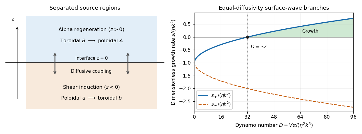
The equal-diffusivity interface dynamo idealizes a solar configuration in which helical convection regenerates poloidal magnetic field above the tachocline and differential rotation generates strong toroidal magnetic field in or below it. Diffusion communicates the fields between the two regions, closing the feedback loop. This separation is the mechanism emphasized by Parker's interface-wave model. An oscillatory traveling mode gives migrating magnetic patterns and polarity reversals; buoyant toroidal flux can appear as sunspot belts. If $x$ is a local latitude coordinate, the direction of their migration depends on the alpha–shear sign and the coordinate orientation.

The magnetic period of this branch is $2\pi /|\omega |$; polarity reverses after half a period, and activity that depends on field strength rather than sign can repeat on that half-period. This is the qualitative relation between the magnetic solar cycle and its activity cycle. The model does not itself predict the observed period or guarantee equatorward migration: those require actual geometry, transport coefficients and shear signs. Real stars also have diffusivity contrasts, meridional transport, spatially varying regeneration and nonlinear feedback. The kinematic exponential mode describes onset, while saturation and a maintained finite-amplitude cycle require further physics.

Use the method of multiple scales, treating $t$ and $\tau =t/ϵ$ as independent variables, so differentiation becomes ${\partial }_t+{ϵ}^{-1}{\partial }_{\tau }$. Write $L={\partial }_x^2-{\ell }^2$ and average over a fast period $2\pi /|\omega |$, with $\omega \ne 0$. The fluctuations can depend slowly on $x,t$ as well as periodically on $\tau$. The ${ϵ}^{-1}$ balance in the poloidal magnetic field potential equation isIntegrating and imposing zero fast average determinesAt order one, the toroidal magnetic field equation is ${\partial }_t\overline{B}+{\partial }_{\tau }\tilde{B}=\Omega {\partial }_x(\overline{A}+\tilde{A})+L\overline{B}$. Its average and fluctuating parts give, respectively,Consequently the zero-average fluctuation isThe order-one averaged poloidal magnetic field potential equation retains the correlation between the fluctuating alpha effect and the fluctuating toroidal magnetic field. Although alpha has zero average, its product with the magnetic fluctuation does not:Thus the rapidly fluctuating alpha effect produces the leading averaged equationsA higher-order zero-average correction to $A$ accommodates the remaining fast order-one terms; it does not alter this leading averaged balance. These equations describe the small-$ϵ$ limit, rather than an exact finite-$ϵ$ identity.

For a Fourier mode, let $(\overline{A},\overline{B})=(a,b)e^{ikx+\sigma t}$ and put $d=k^2+{\ell }^2$. Then $(\sigma +d)a=-ikCb$ and $(\sigma +d)b=ik\Omega a$. Their determinant gives the dispersion relationHere $\Omega C={\Omega }^2{\alpha }_0^2/(2{\omega }^2)\ge 0$, so both growth rates are real. For a prescribed nonzero wavenumber, growth requires $\Omega C>(k^2+{\ell }^2{)}^2/k^2$. If real wavenumbers can be chosen freely, the largest growth rate occurs at $|k|=\sqrt{\Omega C}/2$ and is $\Omega C/4-{\ell }^2$. Hence growing averaged modes exist precisely whenA bounded or periodic spatial domain instead requires an admissible wavenumber satisfying the preceding mode-by-mode inequality.

The physical feedback differs from an ordinary Parker dynamo wave. A constant alpha effect couples $B$ directly into $A$, while the Omega effect differentiates $A$ once, producing the factor $ik\alpha \Omega$ responsible for an oscillatory phase. Here the fast alpha effect first creates a potential fluctuation in temporal quadrature; shear creates a magnetic fluctuation correlated with alpha. The averaged feedback is consequently proportional to $-{\partial }_x\overline{B}$. Combining its spatial derivative with the derivative in the Omega effect gives the real positive factor $\Omega C{k}^2$. In fact $({\partial }_t-L{)}^2\overline{B}=-\Omega C{\partial }_x^2\overline{B}$. The resulting growing fields have fixed spatial phase, so the leading averaged pattern grows without travelling. Fast within-period oscillations of the original fields remain present.

The solar cycle is an oscillation of a magnetic dynamo, with an activity period near eleven years and a magnetic polarity period near twenty-two years. The observational task is to explain a structured, variable cycle rather than a perfectly periodic reversal of one uniform field. Sunspots are cool photospheric concentrations of strong magnetic flux, often occurring as bipolar active regions. Their number rises and falls through successive solar cycles. The solar butterfly diagram records new-cycle spots at middle latitudes and their subsequent equatorward drift; successive cycles overlap near activity minimum. Cycle lengths and amplitudes vary, and the two hemispheres need not evolve in exact synchrony.

Magnetic observations impose stronger constraints than the spot count alone. Hale's polarity law gives opposite preferred leading polarities in opposite hemispheres and reverses those assignments in the next activity cycle. Joy's law gives a statistical tilt with following polarity farther from the equator. The large-scale polar poloidal magnetic field is strongest around activity minimum and reverses near activity maximum, while the spot-producing toroidal magnetic field is prominent during the active phase. Poleward transport of dispersed active-region flux accompanies these polar reversals. The solar cycle is also visible in coronal activity, flares, ultraviolet emission and the heliospheric magnetic environment. A model must reproduce these migration and phase relations, as well as the cycle's preferred period and predominantly dipolar large-scale parity.

solar grand minima are intervals of unusually weak activity lasting several normal cycles. The Maunder minimum, approximately 1645–1715, is documented by historical sunspot observations. Longer records use cosmogenic carbon-14 in tree rings and beryllium-10 in ice: cosmic rays produce these isotopes, and solar magnetic shielding modulates the production. Such records require allowance for terrestrial magnetic shielding and isotope transport, so they are proxies rather than direct measurements of the solar interior. Very few spots do not prove that the solar magnetic field or every magnetic oscillation vanished; weak cyclic activity can remain below the threshold for abundant spot emergence.

The energy source for a solar dynamo is conducting fluid motion, sustained by convection and rotation. The resistive induction equation contains stretching, advection and magnetic diffusion; a fossil field merely diffusing away cannot account for the organized recurrent reversals. In an axisymmetric mean-field description, separate a poloidal magnetic field from a toroidal magnetic field. Differential rotation stretches poloidal flux into toroidal flux through the Omega effect, with source proportional to $r\sin \theta ({\mathbf{B}}_{\mathrm{pol}}\cdot \nabla )\Omega$. This alone cannot complete a self-sustaining regeneration loop. Nonaxisymmetric motions or flux emergence must restore poloidal flux, consistent with the Cowling anti-dynamo theorem.

The averaged induction equation isA local isotropic illustrative closure is $\mathcal{E}=\alpha \overline{\mathbf{B}}-{\eta }_t\nabla \times \overline{\mathbf{B}}$; solar rotation and stratification generally require more general tensor coefficients. Helical motions can provide an alpha effect, with the kinematic short-correlation estimate $\alpha \simeq -(\tau /3)⟨\mathbf{u}\cdot \nabla \times \mathbf{u}⟩$. Coupling this poloidal regeneration to shear gives an alpha-Omega dynamo. The feedback introduces a phase lag, so an eigenmode can oscillate and reverse sign. Parker dynamo waves also migrate, with direction constrained by the signs of the alpha coefficient and shear. Producing equatorward rather than poleward migration is therefore a physical test of the chosen source and rotation profile, not an automatic consequence of any oscillatory solution.

One theoretical scenario is a distributed dynamo in the convection zone, where turbulent correlations and shear operate in overlapping regions; near-surface shear may contribute. Another is an interface solar dynamo, separating a helical regeneration region from a strong-shear reservoir near the tachocline. The rotational transition and stable layer offer possible toroidal-field amplification and storage, but transporting field between separated regions is essential. Flux-tube or magnetohydrodynamic instabilities can supply alternative regeneration processes. Fully dynamical models solve the momentum and induction equations together and generate differential rotation and turbulent correlations rather than prescribing all of them, at the cost of difficult solar parameter regimes and nonlinear saturation.

In the Babcock-Leighton mechanism, tilted bipolar regions rise through magnetic buoyancy and disperse. Their systematically separated polarities undergo different cancellation and transport: following-polarity flux reaching the poles helps reverse and rebuild the polar field. This makes the observed tilt a source of poloidal regeneration and links surface processes to interior toroidal flux. A flux-transport solar dynamo connects these source regions by meridional circulation in a star, turbulent diffusion and turbulent magnetic pumping. Poleward surface transport and an assumed equatorward deep return can help explain the opposite migration of polar and spot-bearing fields. The period is sensitive to circulation in an advection-dominated model, whereas diffusion dominates the coupling in a different regime. Thus similar observed cycles may arise from different transport assumptions.

A linear growing dynamo must be saturated. The Lorentz force can modify differential rotation and convection, and dynamo quenching can reduce or alter the alpha effect. Magnetic-helicity constraints couple the large-scale and fluctuating fields; transport of helicity can matter for avoiding excessively strong quenching. Random variations of active-region tilts or turbulent coefficients produce amplitude fluctuations. Nonlinear mode competition and deterministic modulation can also produce weak epochs, while stochastic or internally generated intermittency can move a dynamo close to or below its excitation threshold. These are competing explanations for solar grand minima. A successful scenario must explain recovery as well as suppression: a poloidal source that depends entirely on large emerging spots becomes weak precisely when those spots disappear, so recovery may require a residual weak-field regeneration mechanism. Observed hemispheric asymmetry and persistence or loss of cycle phase during a weak epoch offer ways to distinguish the scenarios. The observations establish an organized magnetic cycle; they do not select one unique combination of source location, transport and nonlinear modulation.

Write $m_0={\mu }_0\rho$ and treat the imposed mean magnetic field as uniform on the forcing scale. In first-order smoothing, retain terms linear in the fluctuating fields in their equations, while keeping their quadratic correlation when calculating the mean-field electromotive force. The inertial fluctuation, nonlinear induction term and quadratic fluctuating Lorentz force density are neglected in the steady response. The linear magnetic force isAbsorb the gradient into the total pressure. The resulting equations arewith $\nabla \cdot \mathbf{u}=\nabla \cdot \mathbf{b}=0$. Taking the divergence of the first equation gives ${\nabla }^{2}P=0$ for solenoidal forcing. In a periodic or homogeneous Fourier calculation its nonconstant part therefore vanishes.

For each Fourier mode with wavevector $\mathbf{q}$, $|\mathbf{q}|=k$, define $\ell =\mathbf{B}\cdot \mathbf{q}$ andSolving the two coupled linear equations gives the monochromatic coupled magnetic and velocity responseThe magnetic coupling suppresses modes with large projection of their wavevector along the imposed field.

To calculate the mean-field electromotive force, group each pair of opposite wavevectors into a real mode and average its spatial phase. Put $\mathbf{n}=\mathbf{q}/k$, and define its forcing correlationsFor any solenoidal real mode $\mathbf{v}=\mathbf{a}\cos (\mathbf{q}\cdot \mathbf{x})+\mathbf{c}\sin (\mathbf{q}\cdot \mathbf{x})$, its two amplitude vectors are perpendicular to $\mathbf{q}$. Direct multiplication givesAlso, integration by parts gives $⟨(L\mathbf{g})\times (L\mathbf{f})⟩=-{\ell }^2⟨\mathbf{f}\times \mathbf{g}⟩$, where $L=\mathbf{B}\cdot \nabla$. Expanding the response products therefore yieldsSumming over independent real modes, or integrating over their angular spectrum, is the required general answer for $⟨\mathbf{u}\times \mathbf{b}⟩$.

At zero field, $\mathcal{E}(0)={\sum }_{\mathbf{q}}{\mathbf{C}}_{\mathbf{q}}/(\nu \eta k^4)$. Thus the stated zero-field condition removes the unweighted sum of the cross correlations. For anisotropic correlated forcing it does not necessarily remove their differently weighted sum at nonzero field. The displayed general formula retains that allowed contribution. It disappears if cross forcing is absent mode by mode, or under the jointly isotropic statistics assumed for the final part.

The helicity content can also be expressed directly using the actual fluctuating fields. Define their kinetic helicity $H_u(\mathbf{q})=⟨{\mathbf{u}}_{\mathbf{q}}\cdot \nabla \times {\mathbf{u}}_{\mathbf{q}}⟩$ and current helicity $H_b(\mathbf{q})=⟨{\mathbf{b}}_{\mathbf{q}}\cdot \nabla \times {\mathbf{b}}_{\mathbf{q}}⟩$. Substitute $\mathbf{f}=\nu k^2\mathbf{u}-L\mathbf{b}/m_0$ and $\mathbf{g}=\eta k^2\mathbf{b}-L\mathbf{u}$ into their cross correlation. This gives the exact identityIt shows the competing kinetic and magnetic contributions without introducing a spurious singularity when the factor on the left vanishes. For a monochromatic field, ${\mathbf{a}}_b=\nabla \times \mathbf{b}/k^2$ is a magnetic vector potential, so $H_b=k^2⟨{\mathbf{a}}_b\cdot \mathbf{b}⟩$: current helicity is $k^2$ times magnetic helicity. In the isotropic weak-field limit, with zero-field fluctuations ${\mathbf{u}}_0,{\mathbf{b}}_0$, the scalar alpha effect isThis identifies both signs and their different viscous and magnetic relaxation times.

For jointly isotropic forcing let $h_f,h_g$ now denote the total forcing helicities, and set $S_h=\nu h_g/m_0-\eta h_f$. The cross-forcing contribution is even in $\mathbf{B}$, whereas isotropy requires any vector depending only on $\mathbf{B}$ to be parallel to it and odd under reversal. Hence that contribution vanishes. A natural symmetric alpha tensor isOnly its longitudinal coefficient contributes to $\mathcal{E}={\alpha }_{\parallel }\mathbf{B}$. Introduce $h=|B|/[k\sqrt{m_0\nu \eta }]$ and $A_0=\nu \eta k^4$. Angular integration givesTherefore the strong-field quenching of an isotropic electromotive force isprovided $S_h\ne 0$. If the two helicity contributions cancel exactly, this electromotive force vanishes.

There is a tensor qualification to the printed scaling claim. The natural transverse coefficient instead contains $\frac{1}{2}{\int }_0^1(1-{\mu }^2)(1+h^2{\mu }^2{)}^{-2}d\mu \sim \pi /(8h)$ and scales as $|B{|}^{-1}$. The relation ${\mathcal{E}}_i={\alpha }_{ij}{B}_j$ by itself leaves transverse components undetermined. One may choose the effective representative ${\alpha }_{ij}={\alpha }_{\parallel }{\delta }_{ij}$, for which the requested $|B{|}^{-3}$ scaling holds. It is the observable longitudinal response that is fixed, rather than every component of a unique field-dependent tensor.

Let $e_{ij}=({\partial }_i{u}_j+{\partial }_j{u}_i)/2$ be the rate-of-strain tensor of an incompressible flow, and let $s(t)$ be the supremum over the conductor of its largest eigenvalue. State Backus' necessary condition for dynamo action with its magnetic boundary conditions: an isolated bounded conductor of uniform positive magnetic diffusivity $\eta$, surrounded by an electrical insulator with a decaying potential exterior field, and no imposed magnetic field or boundary energy input. For definiteness take a no-slip boundary condition on the fluid, which eliminates the stretching surface term. If the conductor lies within a sphere of radius $R$ and $S={\sup }_{t}s(t)$, a necessary condition for a nondecaying dynamo isThe constant is the free-decay spectral bound for an insulating exterior, not a universal constant for every magnetic boundary condition. The condition is necessary, not sufficient, and involves maximum stretching rather than an rms velocity.

To see both the condition and the growth-rate bound, include exterior magnetic energy:This follows from the resistive induction equation and integration by parts, with the stated boundary assumptions. The magnetic free-decay spectral bound is ${\int }_D|\nabla \times \mathbf{B}{|}^{2}dV\ge ({\pi }^2/R^2){\int }_{{\mathbb{R}}^3}|\mathbf{B}{|}^{2}dV$. For a sphere its lowest mode is the dipolar poloidal free-decay mode; enclosing a smaller conductor gives the same valid lower bound. Since $B_i{e}_{ij}{B}_j\le s(t)|\mathbf{B}{|}^2$, we obtainIntegrating this differential inequality gives decay whenever $S<\eta {\pi }^2/R^2$. More generally the exponential rate of the field norm, rather than of its squared energy, satisfiesSimply discarding the nonnegative resistive dissipation already proves the requested maximum-strain bound. The energy exponent is twice the field-amplitude exponent.

For the alpha-Omega dynamo model, write $a=|{\alpha }_0|$, $w=|\Omega |$, $k\ge 0$ and $d=\eta k^2$. Direct differentiation givesFor $a,kw>0$, use the weighted energy estimate for two coupled modes and form the positive weighted norm $N=kw|A{|}^2+a|B{|}^2$. The inequality $N\ge 2\sqrt{akw}|A||B|$ givesFor each fixed $k$ and model parameters, this norm is equivalent to the amplitude norm; its square-root exponential rate is therefore bounded by $h(k)=\sqrt{awk}-\eta k^2$, uniformly over all admissible $f(t)$. Maximizing over $k$ givesThe exponent is also achievable in order of magnitude. Choose the admissible constant $f=1$. The growing eigenvalue of the two-component system has real part $-\eta k^2+\sqrt{awk/2}$. Its maximum occurs at $k=(aw/(32{\eta }^2){)}^{1/3}$ and equals $32^{-10/3}(a^2{w}^2/\eta {)}^{1/3}$. Thus the bounded-modulation alpha-Omega growth estimate has the scalingThis means the maximum over allowed modulations and wavenumbers, not that every bounded modulation grows; $f=0$ supplies no regenerating alpha coupling.

The Omega effect rapidly makes toroidal field from poloidal field, but exponential dynamo action also requires the slower alpha effect to regenerate the poloidal component. The coupled amplification rate is of order $\sqrt{a\Omega k}$ rather than $\Omega$; shortening the wavelength to increase it also increases magnetic diffusion as $\eta k^2$. Their optimal balance gives $k\sim {\Omega }^{1/3}$ and growth $\sim {\Omega }^{2/3}$. The Backus' necessary condition for dynamo action estimate controls stretching alone and does not incorporate this regeneration bottleneck. A shear without regeneration can give transient amplification but not this sustained exponential feedback.

During the positive half-period, write $Y=(A,B{)}^T$ and $\dot{Y}=K_{+}Y$, with $K_{+}=\left(\begin{array}{cc}0& D^2\\ i& 0\end{array}\right)$. Then $K_{+}^2=i{D}^{2}I={\sigma }^{2}I$. Its two eigenvalues are $\pm \sigma$, and corresponding eigenvectors are $(\sigma ,i{)}^T$ and $(-\sigma ,i{)}^T$. Since $D>0$, they are independent. Thus the general half-period solution isUsing the even and odd terms in the matrix exponential, $e^{T{K}_{+}}=I\cosh (\sigma T)+(K_{+}/\sigma )\sinh (\sigma T)$. Because $D^2/\sigma =-i\sigma$, the fundamental matrix of a linear differential equation givesThe lower-left denominator is $\sigma$, as printed in the PDF. In the negative half-period $K_{-}=\left(\begin{array}{cc}0& -D^2\\ i& 0\end{array}\right)$ and $K_{-}^2=({\sigma }^{\ast }{)}^{2}I$. The analogous matrix exponential has the stated $M^{-}$, replacing $\sigma$ by its complex conjugate ${\sigma }^{\ast }=-i\sigma$. Both matrices satisfywith ${\sigma }^{\ast }$ in the second determinant. Equivalently, their generators have zero trace, so the determinant of each matrix exponential is one.

At each complete period the state is multiplied by the monodromy matrix of a periodic linear system $N=M^{-}{M}^{+}$, so $Y(2nT)=N^{n}Y(0)$. The determinant is therefore $\det N=1$. Let $c_{\pm }=\cosh ({\sigma }^{(\ast )}T)$ and $s_{\pm }=\sinh ({\sigma }^{(\ast )}T)$. Multiplying the two matrices and taking the trace givesThe ratio sum vanishes because the two ratios are $-i$ and $i$. With $x=\sqrt{2}DT$, the hyperbolic-function identity for $|\cosh (a+ia){|}^2$ consequently yieldsFor $x>0$, $F>2$: differentiating gives $F^{\prime }=\sinh x-\sin x>0$, since this derivative has derivative $\cosh x-\cos x>0$ and vanishes initially. The characteristic polynomial is ${\lambda }^2-F\lambda +1$. Hence the two Floquet multipliers are positive, distinct and reciprocal, with dominant multiplier and growth rateThe finite-time propagation within each half-period is bounded independently of the number of cycles, so it does not change this asymptotic Floquet growth rate. The expression is the maximal rate, attained for generic nonzero initial data. The exceptional initial state in the reciprocal multiplier's eigenspace decays with rate $-\gamma$; the zero state stays zero. Thus a vanishing mean alpha effect does not preclude dynamo action in this periodically switched Parker dynamo wave model.

As $x\to \infty$, $F=\frac{1}{2}{e}^x[1+O(e^{-x})]$, $\Lambda =F[1+O(F^{-2})]$, and $\log \Lambda =x-\log 2+o(1)$. ThereforeIn particular, at $T=1$ the rate is asymptotic to $(\sqrt{2}D-\log 2)/2$, as required. The growth calculation uses the product $M^{-}{M}^{+}$, rather than averaging the two generators: the two generators do not commute.

Under the first-order smoothing approximation, neglect the fluctuating product in the resistive induction equation while retaining its contribution to the mean electromotive force. Since the test field ${\mathbf{B}}_0$ is constant and the velocity is a solenoidal vector field, the fluctuation equation isLet $a=\eta k^2>0$, $d=a^2+{\Omega }^2$, and ${\mathbf{C}}_j=i({\mathbf{B}}_0\cdot {\mathbf{k}}_j){\hat{\mathbf{u}}}_j$. For each Fourier mode, the diffusion equation becomes a scalar linear relaxation equation applied to each vector component. Take its long-time periodic response, with $\Omega \ne 0$. For the first mode,while for the second,Thus the complex response coefficients areThey giveAn arbitrary initial fluctuation also contains a homogeneous diffusive transient. In the forced modes this is $\mathrm{Re}{\sum }_j{\mathbf{r}}_j{e}^{i{\mathbf{k}}_j\cdot \mathbf{x}-at}$; more general initial modes also diffuse. The displayed harmonic expression is the periodic particular solution after those transients, not the most general solution at finite time. The constants $a,d$ and the factors of $i$ are unchanged by taking the final real part.

To justify the helicity relation, write ${\hat{\mathbf{u}}}_j={\mathbf{a}}_j+i{\mathbf{c}}_j$ with real vectors. Solenoidality gives ${\mathbf{k}}_j\cdot {\mathbf{a}}_j={\mathbf{k}}_j\cdot {\mathbf{c}}_j=0$. Their cross product is parallel to ${\mathbf{k}}_j$, andThis is the helicity vector of a solenoidal Fourier mode. In these conventions the spatially averaged kinetic helicity density of $\mathrm{Re}({\hat{\mathbf{u}}}_j{e}^{i{\mathbf{k}}_j\cdot \mathbf{x}})$ is $-H_j{k}^2$; the sign is set by the specified cross-product order.

For equal wavevectors, spatial averaging of two real harmonic fields givesTime averaging gives another factor $1/2$, because $⟨{\cos }^2\Omega t{⟩}_t=⟨{\sin }^2\Omega t{⟩}_t=1/2$ and the mixed temporal average is zero. Consequently each diagonal mode contributes to the mean-field electromotive forceDistinct modes with ${\mathbf{k}}_1\ne \pm {\mathbf{k}}_2$ have no spatially averaged cross term. The printed condition also permits the opposite-wavevector case. The possible cross terms still cancel after time averaging: the out-of-phase response coefficients are ${\mathbf{p}}_2=-\Omega {\mathbf{C}}_2/d$ and ${\mathbf{q}}_1=\Omega {\mathbf{C}}_1/d$, while integration by parts gives $⟨{\mathbf{u}}_1\times ({\mathbf{B}}_0\cdot \nabla ){\mathbf{u}}_2{⟩}_x=⟨{\mathbf{u}}_2\times ({\mathbf{B}}_0\cdot \nabla ){\mathbf{u}}_1{⟩}_x$ for the real spatial fields. This handles all the distinct wavevectors allowed by the question, assuming the usual periodic-cell or whole-space spatial average.

Thus the alpha tensor isBoth averaging factors matter. The alpha tensor is real and symmetric, and this contribution vanishes when the mode kinetic helicity densities vanish.

For the two perpendicular wavevectors and common $H_1=H_2=H$, put ${\alpha }_0=\eta H{k}^4/[2({\Omega }^2+{\eta }^2{k}^4)]$. ThenMean-field dynamo action is possible when ${\alpha }_0\ne 0$ and sufficiently long mean-field wavelengths are allowed. The missing $zz$ entry does not prevent an alpha-squared dynamo. Indeed a slowly varying mean magnetic field transverse to $z$, with dependence $e^{iKz+\lambda t}$, obeysThe two growth rates are $-\eta K^2\pm {\alpha }_{0}K$, so the larger is positive if $0<|K|<|{\alpha }_0|/\eta$. This supplies a brief constructive reason; scale separation also requires $|K|\ll k$. A spatially uniform test field itself has zero curl of its mean-field electromotive force and does not grow. If $H=0$, or if boundary conditions exclude all unstable long wavelengths, this particular alpha effect does not yield growth. The conclusion concerns the stated first-order smoothing approximation; no uncomputed turbulent-diffusion correction is assumed.

In a Parker dynamo wave model, an alpha effect of the form $\alpha ={ϵ}^{-1}{\alpha }_0\sin (\omega t/ϵ)$ has zero time average but can generate a finite averaged coupling. The method of multiple scales gives $\tilde{A}=-({\alpha }_0/\omega )\cos (\omega \tau )\overline{B}$ and $\tilde{B}=-(\Omega {\alpha }_0/{\omega }^2)\sin (\omega \tau ){\partial }_x\overline{B}$, where $\tau =t/ϵ$. Consequently $C=\Omega {\alpha }_0^2/(2{\omega }^2)$. With diffusion operator ${\partial }_x^2-{\ell }^2$, the averaged Fourier mode growth exponents are $-k^2-{\ell }^2\pm |k|\sqrt{\Omega C}$. For freely adjustable real $k$, growth requires $\Omega C>4{\ell }^2$. The result is an asymptotic averaged model for fixed nonzero $\omega$, not an exact replacement at finite $ϵ$.