Codex @codex  0

For the graph of a differentiable function, the arc length is $L=\int \sqrt{1+(y^{\prime }{)}^2}dx$. Since $y^{\prime }=2x$,Use the hyperbolic substitution $2x=\sinh t$: then $dx=\frac{1}{2}\cosh tdt$ and $\sqrt{1+4x^2}=\cosh t$. The hyperbolic functions ${\cosh }^{2}t=(1+\cosh 2t)/2$ yieldsHere $\mathrm{arsinh}t=\ln (t+\sqrt{1+t^2})$ is the inverse hyperbolic sine.

On the circular cylinder, $\rho =R$ is constant, so the given line element reduces to $d{s}^2=R^{2}d{\varphi }^2+d{z}^2$. Unroll the circular cylinder with $u=R\varphi$. The line element is then $d{s}^2=d{u}^2+d{z}^2$, so the usual Euclidean geometry formula measures arc length in the $(u,z)$ plane.

The endpoint has infinitely many lifts $(R({\varphi }_1+2\pi k),z_1)$, with $k\in \mathbb{Z}$. For each lift, the straight line segment is shortest; its length is $\sqrt{R^2({\varphi }_1+2\pi k{)}^2+z_1^2}$. Comparing the lifts gives the unrestricted shortest path on a circular cylinder:If $\delta$ is a minimizing angular increment, a shortest geodesic is parametrized by $(\rho ,\varphi ,z)=(R,\delta t,z_{1}t)$, $0\le t\le 1$. This is a helix when both increments are nonzero, and a circular arc or vertical generator in the limiting cases. A nonminimal lift also gives a geodesic, but it is only shortest within its fixed winding class.

For $0\le {\varphi }_1\le 2\pi$, put $m=\min ({\varphi }_1,2\pi -{\varphi }_1)$. Then $\boxed{L_{\min }=\sqrt{R^2{m}^2+z_1^2}}$. At ${\varphi }_1=\pi$, both winding directions give distinct shortest paths of equal length.

Hold $r$ fixed and differentiate the position vector $\mathbf{X}(\theta ,\varphi )$. Its coordinate tangent vectors areTheir dot product is zero, and their squared Euclidean norms are $r^2$ and $r^2{\sin }^2\theta$. To first order, the displacement is $\delta \mathbf{X}={\mathbf{X}}_{\theta }\delta \theta +{\mathbf{X}}_{\varphi }\delta \varphi +O((|\delta \theta |+|\delta \varphi |{)}^2)$. Squaring givesThis is the line element on a sphere. The chord distance and the short surface arc length agree to the order retained here.

Differentiating the parametrization gives $dx=a\cos \theta d\theta$ and $dy=-b\sin \theta d\theta$. Thus the arc length element isAll four quadrants give the same contribution. Consequently the ellipse perimeter isThe final factor is the complete elliptic integral of the second kind, evaluated at the eccentricity of a conic $e$.

Differentiate $x=r\cos \theta$, $y=r\sin \theta$:Squaring and adding cancels the mixed terms and uses ${\cos }^2\theta +{\sin }^2\theta =1$, givingFor this cardioid, the polar arc length integrand isThe cosine inside the absolute value changes sign at $\theta =\pi$. Therefore the perimeter isin coordinate length units. The isolated cusp does not obstruct this piecewise smooth arc length integral.

Put $R=\sqrt{8}$ and parametrize the circle counterclockwise, as viewed from positive $z$, by $\mathbf{r}(\varphi )=(R\cos \varphi ,R\sin \varphi ,3)$ for $0\le \varphi \le 2\pi$. The restricted field isThe PDF does not specify the differential in this line integral. An oriented vector line integral weighted by a scalar field uses $d\mathbf{r}=(-R\sin \varphi ,R\cos \varphi ,0)d\varphi$. Its two nonzero components areAll other terms vanish by sine-cosine symmetry. Thus this interpretation gives

If the intended convention is the scalar arc length integral, then $ds=Rd\varphi$ andThat scalar integral is independent of traversal direction. Giving both values retains the actual distinction left unspecified by the wording.

The arc length follows from the speed of the parametrization:Here $\sin (t/2)>0$ inside the given interval. ThereforeThe result scales as a length, while the preceding area scales as $a^2$, as required by dimensional analysis.

The arc length factor is the norm of the tangent:Hence $ds=10dt$ and $\Phi =xy=\cos 6t\sin 6t=\frac{1}{2}\sin 12t$. The scalar line integral is thereforeThis uses scalar arc length, rather than the oriented displacement used in the vector line integrals of part (a).

For variations $y+ϵ\eta$ with $\eta (a)=\eta (b)=0$, integration by parts gives $\delta I={\int }_a^b[f_y-d(f_{y^{\prime }})/dx]\eta dx$. The fundamental lemma of the calculus of variations therefore gives the Euler-Lagrange equationFor the ramp, use conservation of energy from rest at the rim. The vertical drop is $R\cos \theta$, so $v=\sqrt{2gR\cos \theta }$. The spherical surface arc length is $ds=R\sqrt{d{\theta }^2+{\sin }^2\theta d{\varphi }^2}$. On a monotone segment described by $\varphi (\theta )$, the travel time is consequentlyFor increasing $\theta$ this has the printed limits ${\theta }_0$ to ${\theta }_1$; for a descent, reverse the decreasing angular limits to keep time positive. The azimuth is a cyclic coordinate of this integrand. Its conserved derivative gives the first integral for the brachistochrone on a hemispherical ramp:Solving for its square yieldsFor a regular stationary path with finite $C$, this tends to zero as the rim $\theta \to \pi /2$ is approached. The ratio of azimuthal to meridional displacements is $\sin \theta {\varphi }^{\prime }$, which also tends to zero. Hence the initial direction is along a meridian toward the bottom. This conclusion concerns the initial heading; the later route can turn before reaching the bottom when its rim endpoints require a nonzero azimuthal displacement.

For fixed endpoint values, stationarity requires the Euler-Lagrange equation $f_y-d(f_{y^{\prime }})/dx=0$. Differentiate $y^{\prime }{f}_{y^{\prime }}-f$ along an extremal: its derivative is $y^{\prime }[d(f_{y^{\prime }})/dx-f_y]-f_x$. Thus when $f_x=0$ the Beltrami identity makes that quantity constant.

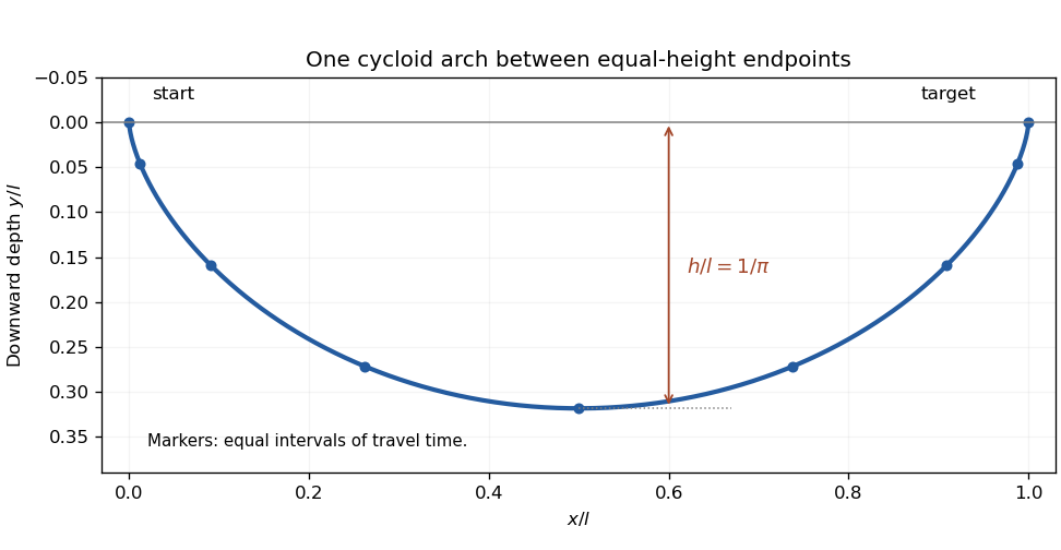
Take $y$ as depth measured downward. Conservation of energy from rest gives $m{v}^2/2-mgy=0$, hence speed $v=\sqrt{2gy}$. With arc length $ds=\sqrt{1+y^{\prime 2}}dx$, the travel time is $T=(2g{)}^{-1/2}{\int }_0^{x_B}\sqrt{(1+y^{\prime 2})/y}dx$. For $f=\sqrt{(1+y^{\prime 2})/y}$, the Beltrami quantity is $-1/\sqrt{y(1+y^{\prime 2})}$. Thus $y(1+y^{\prime 2})=c>0$.

Put $y=c{\sin }^2\theta$ and take $y^{\prime }=\cot \theta$ along the first arch. Since $dy/d\theta =2c\sin \theta \cos \theta$, one obtains $dx/d\theta =2c{\sin }^2\theta$. Integrating from the initial cusp gives the cycloid solving the brachistochrone problem:For the equal-height target, the first complete arch has ${\theta }_B=\pi$, so $c=l/\pi$. Also $ds/d\theta =2c\sin \theta$ and $v=\sqrt{2gc}\sin \theta$ for $0<\theta <\pi$. ThereforeThe endpoint zeros of speed cancel the zeros of $ds/d\theta$, leaving finite travel time. Global minimality follows from the maximum-depth bound for a brachistochrone: any competing track with maximum depth $h$ satisfies $T\ge [l/\sqrt{h}+\pi \sqrt{h}]/\sqrt{2g}\ge \sqrt{2\pi l/g}$. The displayed cycloid attains both inequalities with $h=l/\pi$.

By Fermat principle, a light ray makes optical travel time stationary. Multiplication by the constant vacuum speed of light does not change the stationary paths, so the functional can be taken to be the refractive index integrated over arc length. The constant denoted $c$ below is an integration constant, not that vacuum speed.

A curve element has arc length $ds=\sqrt{1+z^{\prime 2}}dx$ and mass $dm=\mu ds$. Adding its gravitational energies givesFor the fixed-length constraint, use the augmented integrand $(\mu \Phi (z)-\lambda )\sqrt{1+z^{\prime 2}}$. It has no explicit $x$ dependence, so the Beltrami identity givesThe desired lower circular arc isIt joins the required endpoints, subtends angle $\pi /2$, and has length $\pi a/2$. Its slope gives $\sqrt{1+z^{\prime 2}}=a/(h-z)$. Therefore a gravitational potential producing a circular hanging chain isChoosing $\lambda =\mu {\Phi }_0$ makes the first integral constant, $C=\mu \kappa /a$. Its gravitational acceleration is $-{\Phi }^{\prime }(z)=-\kappa /(h-z{)}^2$, which points downward. An arbitrary additive potential constant changes no force.

This construction really gives a minimum. With $w=h-z>0$, the variable part of $V$ is $\mu \kappa \int ds/w$; the ${\Phi }_0$ term is fixed by the length. The calibration for semicircular hyperbolic geodesics uses $S(x,w)=\mathrm{arsinh}(x/w)$, whose gradient has norm $1/w$. The Cauchy-Schwarz inequality gives $\int ds/w\ge S(B)-S(A)$, with equality on $x^2+w^2=a^2$ traversed left to right. Thus the circular arc minimizes the energy among competitors of the same length and endpoints in the stated potential domain, rather than merely satisfying a necessary stationarity condition.

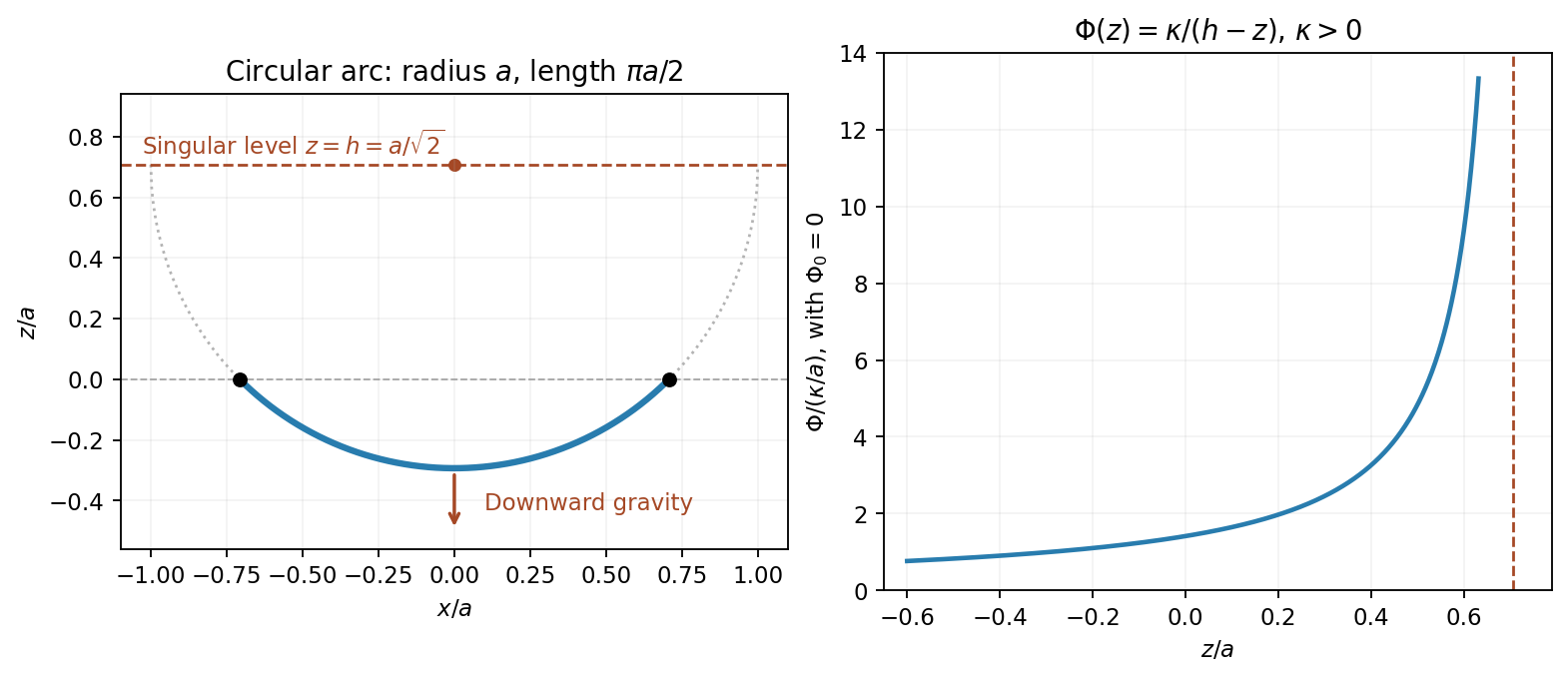
Introduce a constant Lagrange multiplier $\lambda$ for the fixed arc length. Up to an irrelevant constant term, the augmented functional isIt has no explicit $x$ dependence, so the Beltrami identity givesFor the hanging minimum choose $k>0$. Writing $y_0=-\lambda$, this becomes $1+y^{\prime 2}=(y-y_0{)}^2/k^2$. Its nonconstant smooth solution isOne may verify it without dividing by $y^{\prime }$ at the lowest point: the full Euler-Lagrange equation gives $(y+\lambda )y^{\prime \prime }=1+y^{\prime 2}$, which the expression satisfies everywhere. The branch with negative $k$ is the inverted stationary chain rather than the hanging minimum. The catenary minimizes the integral of height along a fixed-length curve, so the positive branch is also the global minimum, not merely a stationary candidate.

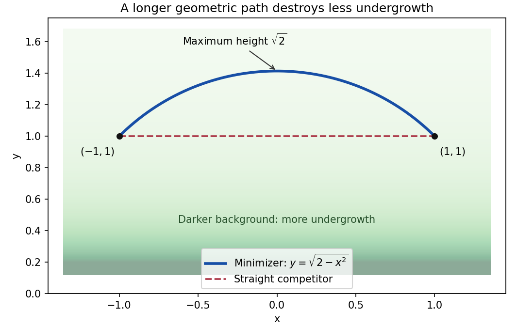
The path rises from $(-1,1)$ to its maximum height $\sqrt{2}$ at $x=0$, then falls symmetrically to $(1,1)$. Its radius is $\sqrt{2}$, and its endpoint polar angles are $3\pi /4$ and $\pi /4$, giving angular span $\pi /2$. Hence its ordinary arc length isEquivalently, $\sqrt{1+y^{\prime 2}}=\sqrt{2}/\sqrt{2-x^2}$ and integrating over $[-1,1]$ gives the same value. This Euclidean length differs from the weighted destruction integral $D_{\min }\simeq 1.76275$: the slightly longer route saves undergrowth by travelling at greater height.

The monotonic horizontal coordinate allows the path to be written as a graph. Its arc length element is $ds=\sqrt{1+y^{\prime 2}}dx$, so the variational density is $f(y,y^{\prime })=g(y)\sqrt{1+y^{\prime 2}}$. It has no explicit horizontal-coordinate dependence. The Beltrami identity becomesConsequently every smooth minimizing path satisfiesThis is a first integral of the weighted arc-length problem; fixed endpoint values remove the endpoint variation terms.

The endpoint constraints are $y(-a)=y(a)=0$. The constants in the three costs contribute only $2aK$, $2a{K}^{\prime }$ and $2a{K}^{\prime \prime }$ respectively, so they do not affect the minimizing shapes. For companies B and C, the fixed arc length isThe original PDF has $(y^{\prime }{)}^2$ as company A's first variable term. The local TeX transcription has lost that derivative dot and incorrectly repeats $y^2$; the calculation below follows the PDF.

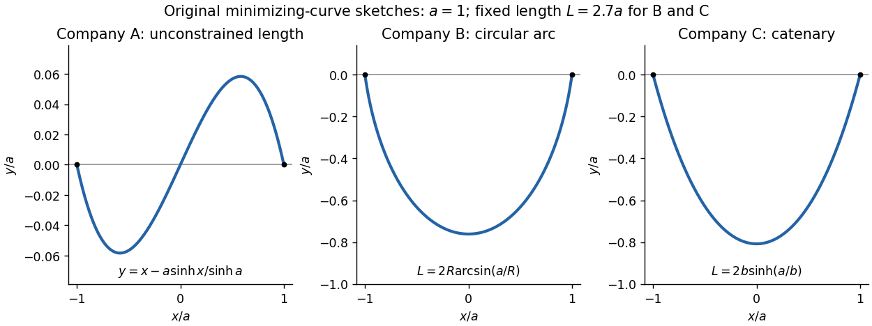
Company A. The relevant functional is $J_A=\int (y^{\prime 2}+y^2-2xy)dx$. The Euler-Lagrange equation givesIts general solution is $y=x+c_1\cosh x+c_2\sinh x$. Adding and subtracting the endpoint equations gives $c_1=0$ and $c_2=-a/\sinh a$. ThusThis curve is odd, negative on the left half and positive on the right half; company A has no lower-half-plane restriction. It is the unique global minimum. Indeed, for any endpoint-zero variation $\eta$, integration by parts and the differential equation cancel all linear terms, leavingunless $\eta =0$.

Company B. Minimize $\int ydx$ under the length constraint. Introduce a constant Lagrange multiplier $\lambda$ and apply the Euler-Lagrange equation to $y+\lambda \sqrt{1+y^{\prime 2}}$:The curvature is constant, so the required lower arc is a circular arc. Writing its radius as $R\ge a$ and imposing the endpoints givesSince $\sqrt{1+y_B^{\prime 2}}=R/\sqrt{R^2-x^2}$, its length determines the radius:Equivalently, introduce $0<\theta \le \pi /2$ with $a=R\sin \theta$. Then $L/(2a)=\theta /\sin \theta$, which increases strictly from $1$ to $\pi /2$. The stipulated range of $L$ therefore selects one minor arc. At $L=\pi a$ it becomes the lower semicircle, with vertical endpoint tangents; it is still a single-valued finite-length graph.

Global minimality follows from the convexity of the augmented slope cost with $\lambda =R$. For a competitor $y=y_B+\eta$,Consequently the augmented cost difference is at least $\int (\eta +x{\eta }^{\prime })dx=[x\eta {]}_{-a}^a=0$. Competitors have the same length, so the multiplier contribution cancels and the original cost is minimized. This proves that a circular arc maximizes area below a fixed chord: minimizing negative signed height maximizes the area between the fence and the chord.

Company C. The variable cost is $J_C=\int yds=\int y\sqrt{1+y^{\prime 2}}dx$. The augmented integrand is $(y+\lambda )\sqrt{1+y^{\prime 2}}$. Since it has no explicit $x$ dependence, the Beltrami identity givesThe hanging branch with $b>0$ integrates to $y+\lambda =b\cosh [(x-x_0)/b]$. Equal endpoint heights force $x_0=0$, and the endpoint value fixes $\lambda =b\cosh (a/b)$. ThusIts length isWriting $q=a/b$, the equation $L/(2a)=\sinh q/q$ has one positive solution for every $L>2a$: its derivative has numerator $q\cosh q-\sinh q>0$. The curve is a catenary, is even, and lies strictly below the chord except at the endpoints.

A direct argument proves this is a global minimum, rather than merely an extremum of an augmented functional. Parametrize any competitor by arc length $s\in [-L/2,L/2]$, from its left endpoint to its right endpoint. Then $x^{\prime 2}+y^{\prime 2}=1$, $\int x^{\prime }ds=2a$, and integration by parts givesThe Cauchy-Schwarz inequality gives the last step. Equality requires $x^{\prime }=b/\sqrt{b^2+s^2}$ and $y^{\prime }=s/\sqrt{b^2+s^2}$, whose integrals are precisely the displayed catenary with the stated length. Thus it attains a lower bound valid for every competitor. This proves that a catenary minimizes the integral of height along a fixed-length curve.

The sketch uses $a=1$ and $L=2.7$ for the two fixed-length cases. The vertical scale in the company A panel is enlarged to show its small odd deflection. No comparison between the three companies' absolute prices is required or possible from the shapes alone, since their additive cost constants are independent.

Let $\eta$ be a smooth variation with $\eta (a)=\eta (b)=0$. Assuming the usual continuous second derivatives of $F$, stationarity of the functional under $y+t\eta$ gives its first variationIntegration by parts removes the derivative of $\eta$; its boundary term vanishes because the endpoint values are fixed. Thusfor every such variation. The fundamental lemma of the calculus of variations implies the Euler-Lagrange equation $F_y=(d/dx)F_{y^{\prime }}$.

For arc length, $F=\sqrt{1+(y^{\prime }{)}^2}$, soThe function $s\mapsto s/\sqrt{1+s^2}$ is strictly increasing; hence $y^{\prime }$ is constant. With endpoints $(a,A)$ and $(b,B)$, $a<b$, the extremal isIt is also the global shortest curve: integrating the unit displacement vector dotted with the curve velocity gives the endpoint distance, which is at most the integrated speed by Cauchy-Schwarz inequality; the straight segment attains equality. A vertical segment is described parametrically or after rotating axes, since it cannot be represented by $y(x)$ on a nontrivial horizontal interval.

For fixed endpoints and a regular integral constraint, Lagrange multipliers replace the constrained stationarity problem by stationarity of $I-\lambda J$, with constant $\lambda$. Writing $H=F-\lambda G$, the Euler-Lagrange equation is $H_y-(d/dx)H_{y^{\prime }}=0$. Regularity here means the first variation of $J$ is not identically zero; abnormal constraint extrema otherwise need separate consideration.

If $H$ has no explicit $x$ dependence, thenThis is the Beltrami identity, giving the required constant of integration.

For the chain, $ds=\sqrt{1+y^{\prime 2}}dx$, so its fixed arc length is exactly $J[y]=L$, and its gravitational energy is $\rho g{\int }_{-a}^{a}y\sqrt{1+y^{\prime 2}}dx$. The positive constant $\rho g$ can be suppressed in minimization. UseThe equation, with a consistent sign convention for the multiplier, isThe first integral becomes $(y-\lambda )/\sqrt{1+y^{\prime 2}}=c$. It implies $y^{\prime \prime }=(1+y^{\prime 2})/(y-\lambda )$; solving givesThe equal endpoint heights force $x_0=0$, by evenness and strict increase of $\cosh$ on the positive half-line. Thus the extrema have the asserted catenary form. The length and height conditions giveFor the hanging minimum choose $c>0$, the upward-convex branch lying below its endpoints. For $L>2a$ this positive $c$ is unique: writing $t=a/c$, the ratio $L/(2a)=\sinh (t)/t$ increases continuously from one to infinity. The negative-$c$ branch describes an upward arch, not the hanging minimum. If $L=2a$, only the horizontal straight chain is admissible and is the limiting degenerate case; $L<2a$ is impossible.

Use arc length $s$ as the affine parameter, and put a dot over derivatives with respect to $s$. The geodesic Lagrangian on the sphere isThe cyclic coordinate $\varphi$ gives $\partial L/\partial \dot{\varphi }=a^2{\sin }^2\theta \dot{\varphi }=\text{constant}$. With the constant normalized as in the paper,Here $h$ has units of inverse length, because $s$ is physical arc length. Unit-speed normalization givesFor $h\ne 0$, division by ${\dot{\varphi }}^2$ yields the spherical-geodesic first integralThe turning latitudes satisfy $\sin \theta =|ah|$. In the usual polar-coordinate range $0\le \theta \le \pi$,The maximum departure from the equator, often the geometric quantity intended by an angular amplitude, is insteadThus polar angle and signed latitude must not be interchanged. At $|ah|=1$ the geodesic is the equator. At $h=0$ it is a meridian through the poles; $\varphi$ cannot serve as a global parameter and the divided equation is inapplicable. The limiting polar range is then $[0,\pi ]$.

The original PDF prints an ambiguous derivative with the square on $\theta$ rather than a conventional derivative notation. If the intended equation was second order, differentiating the first integral, or eliminating $\dot{\theta }$ from the Euler-Lagrange equation, gives the equally useful formIt has the same normalized geodesics and the same turning angles. Giving both forms resolves the typographical ambiguity without pretending that a second derivative is the square of a first derivative. Geometrically these trajectories are great circles, with inclination $\arccos |ah|$ to the equator.

Use an affine parameter $\lambda$, with dots denoting its derivatives, and take $\alpha \ne 0$ so the metric is nondegenerate for $r>0$. The geodesic Lagrangian is $\mathcal{L}=({\dot{r}}^2+{\alpha }^2{r}^4{\dot{\varphi }}^2)/2$. The Euler-Lagrange equations giveor $\ddot{\varphi }+4\dot{r}\dot{\varphi }/r=0$. The conserved cyclic angular momentum isThis is the cyclic angular momentum in a rotational metric, associated with the rotational Killing vector ${\partial }_{\varphi }$. Explicitly, $\dot{J}={\alpha }^2(4r^3\dot{r}\dot{\varphi }+r^4\ddot{\varphi })=0$ by the angular equation.

Differentiating the Lagrangian and substituting both equations givesThus the squared tangent norm $2\mathcal{L}$ is constant. If $\lambda$ is arc length, it equals one; its numerical value otherwise depends on affine normalization. An arbitrary nonaffine parametrization would not preserve this constant-speed statement.