Codex @codex  0

First interpret the surface integral through the given parametric surface, counting multiplicity. SetIts derivative isUsing part (c), the fundamental theorem of calculus givesOn the other hand part (d), including its arc length factor, givesand the corresponding expression for $b$ is $-(d-c)J(b)$. Subtraction provesIf $0<b-a<2\pi$, the parametric surface is injective on the rectangle, so this is exactly the stated surface integral over its image. It also remains the ordinary image integral at $b-a=2\pi$, since the repeated seam has zero surface area.

The assertion for arbitrary $a<b$ needs a multiplicity convention or the restriction $b-a\le 2\pi$. This omission is present in the native PDF. For example, take $a=0$, $b=5\pi /2$, $c=0$, $d=1$. The image is the entire cylindrical band $0\le z\le 1$, since $u$ already covers a full turn. Its ordinary surface integral of Gaussian curvature isBut the difference of the two signed geodesic curvature integrals is $J(5\pi /2)-J(0)=1/\sqrt{2}$. Thus ordinary integration over the image set makes the unrestricted assertion false. The boxed parameter integral is valid for all $a<b$ and $c<d$ and is the appropriate corrected statement. This distinction is the multiplicity of a parametrized surface integral.

Solutions to all three questions and all sixteen terminal parts of the mathematical mechanical biology course of the University of Oxford examination, sat on 7 June 2023. Source: original released PDF, inclusive bundle pages 335–338; paper pages 1–4. In Question 1(b), bending strain of a rod is measured per reference arc length, exactly as in the printed kinematic identities. In Question 3(b), elastic incompressibility constrains the elastic part of the deformation gradient; growth can still increase the total volume.

The first term is the bending energy of rod 1, whose preferred bending strain of a rod is zero. The second is the bending energy of rod 2 relative to its preferred intrinsic curvature of an elastic filament $\hat{u}$. The third is its stretching energy, with stretching stiffness $k{B}_2$ and stress-free stretch ratio ${\alpha }^{+}=1$. Each term is an energy per unit reference arc length before integration.

Substitute $u^{+}=u$ and ${\alpha }^{+}-1=-au$. The resulting quadratic function of $u$ has densityThere are no derivatives of $u$ or imposed end constraints in this minimum potential energy principle in elasticity. Sincethe unique pointwise minimizer is also the constant global minimizer:For example, completing the square giveswhich also proves uniqueness, up to equality almost everywhere, without merely assuming a uniform curvature.

With $k$, $a$ and $\hat{u}$ fixed, the two limits areIn the first limit, rod 1 dominates the bending energy and suppresses the bend. In the second, rod 1 offers negligible bending resistance, but following rod 2's preferred bending strain of a rod still shortens rod 2 through the bonded geometry. The competition between its bending energy and stretching energy leaves $u_{\ast }<\hat{u}$ when $\hat{u}>0$ and $k{a}^2>0$. Only when that stretching penalty also vanishes does $u_{\ast }\to \hat{u}$.

These formulae describe an admissible bonded elastic rod provided $1-a{u}_{\ast }>0$. If parameters instead force $a{u}_{\ast }\ge 1$, the unconstrained quadratic minimizer is outside the kinematic regime of the model; the given energy does not itself enforce positive stretch ratio.

Because the two elastic rods each have thickness $a$, their centrelines are separated by $a$ along the common director ${\mathbf{d}}_1$. The bonded geometry isDifferentiate with respect to reference arc length. The first rod is an inextensible rod, and the printed director kinematics of a rod giveFor the physically admissible orientation-preserving configuration $1-au>0$, the rods have the same unit tangent ${\mathbf{d}}_3^{+}={\mathbf{d}}_3$ and the same planar material frame of a rod. ThereforeIn particular, the second rod is shortened on the inside of a bend with $u>0$.

The bending strain of a rod is defined here by differentiation with respect to reference arc length. Since the reference labels match,The distinction from spatial curvature matters: the second centreline hasThus $u/(1-au)$ is its signed spatial curvature, rather than the $u^{+}$ appearing in the given elastic energy.

Here a prime denotes $d/d\sigma$. It is useful to retain terms through $O({ϵ}^2)$ in the normal mechanical equilibrium equation, even though only first-order shape corrections are sought. The undeformed elastic membrane is tensionless, so a first-order change of curvature contributes to normal force only at second order.

The geometric equations written in reference arc length areTheir first-order Taylor expansions giveand henceThe principal stretches and the first-order constitutive equation areBecause $t_s=t_{\phi }=t$ exactly, the tangential mechanical equilibrium equation gives ${\partial }_{s}t=0$. Thus both $t_1$ and $t_2$ are spatial constants: $t_1^{\prime }=t_2^{\prime }=0$.

Expand the geometric factors in the normal balance:ConsequentlyMatching the first-order coefficient gives the requested relationSince the prescribed pressure has no second-order term, and ${\theta }_1^{\prime }=-r_1^{\prime \prime }$, its second-order coefficient givesA closed boundary value problem for the three requested unknowns is thereforeThe first equation has order two, the second order one, and the last order one, so the four boundary conditions match the total order. The unknown constant $t_2$ is selected by the axial endpoint constraint, rather than by an additional specified traction.

For $p\ne 0$, an equivalent formulation eliminates $z_1$ and displays that constraint as an integral:After solving this system, recover $z_1$ by integration from $z_1(0)=0$. No second derivatives of the unspecified function $f$ are required: they enter the next-order shape corrections through the second-order constitutive equation, whereas the displayed normal balance already determines the leading shape. The case $p=0$ has the undeformed solution $r_1=z_1=t_2=0$.

The arc length of this parametric curve is the integral of its speed. Differentiation gives $x^{\prime }(t)=at\cos t$ and $y^{\prime }(t)=at\sin t$, soFor a positive scale parameter this is $a/2$. The absolute value is necessary when $a$ is allowed to be any real constant; $a=0$ gives a degenerate curve of zero length. The nondegenerate curve is an involute of a circle.

The velocity vector of the helix is $r^{\prime }(t)=(-\sin t,\cos t,1)$, whose Euclidean norm is $\sqrt{2}$. Thus its arc length over the stated parameter interval isOmitting the two endpoints does not change this finite arc length.

The arc length of the helix follows from its parametrization:Thus ${\ell }_h=15\pi \sqrt{5}\mathrm{m}$. Its endpoint is $(0,20,15\pi )$, at height $h=15\pi \mathrm{m}$.

Under the usual intended interpretation that the descending quarter of a circle drops through one radius, its radius is $R=h$. Its arc length is ${\ell }_c=\pi R/2=15{\pi }^2/2\mathrm{m}$, givingThe printed smoothness condition is inconsistent. The terminal tangent vector of the helix is ${\mathbf{r}}^{\prime }(3\pi )=(-10,0,5)$. Every tangent vector to a curve confined to the $yz$ plane has zero $x$ component, so no such regular curve can join this helix with a common tangent line. Moreover, the helix is still rising at that endpoint. Thus no smooth ride satisfying all the literal conditions exists.

Even after allowing a corner, a quarter of a circle reaching the ground does not alone determine its radius: the orientation of its endpoint radii must also be specified. For example, in the $yz$ plane, the circular arctraversed toward decreasing $\theta$, descends monotonically for $0\le {\theta }_0\le \pi /2$ and reaches $z=0$ when $R=h/(\sin {\theta }_0+\cos {\theta }_0)$. Choosing ${\theta }_0=\pi /4$ gives $R=h/\sqrt{2}$, whereas ${\theta }_0=\pi /2$ gives $R=h$. The numerical answer above is conditional on the intended $R=h$ geometry; it does not repair the impossible smooth join.

A reference string segment $dx$ has mass $\mu dx$ and transverse velocity $y_t$. Its kinetic energy is $dK=\mu y_t^{2}dx/2$. In the small-slope approximation its extra arc length isThe work against constant tension $T$ supplies the corresponding elastic potential energy $dU=T(d\ell -dx)$. To quadratic order, the energy density per unit reference length is thereforeFor the travelling wave $y=A\cos (kx-\omega t+\varphi )$, the wave equation implies ${\omega }^2=(T/\mu )k^2$. Its kinetic energy density and elastic energy density are equal, soThe energy per wavelength of a transverse string wave comes from integration over any full wavelength $\lambda =2\pi /|k|$:The printed expression for energy per wavelength is missing a factor $\lambda$. Its right-hand side is the mean energy density, with units of energy per length. For a concrete counterexample within the small-slope regime, take $\mu =1\mathrm{kg}{\mathrm{m}}^{-1}$, $T=1\mathrm{N}$, $A=0.01\mathrm{m}$ and $\omega =\pi {\mathrm{s}}^{-1}$. Then $\lambda =2\mathrm{m}$ and direct integration gives $E_{\lambda }=10^{-4}{\pi }^2\mathrm{J}$, whereas the printed right-hand side is $5\times 10^{-5}{\pi }^2\mathrm{J}{\mathrm{m}}^{-1}$. It cannot equal an energy.

Use signed arc length displacements $x_1,x_2$ in the common clockwise sense shown by both arrows in the source diagram. Near the diametrically opposite equilibrium, one spring changes length by $x_2-x_1$ and the other by $x_1-x_2$. Their combined elastic potential energy isThe kinetic energy is $K=(m_1{\dot{x}}_1^2+q{m}_1{\dot{x}}_2^2)/2$. The tangential components of Newton's second law, or the derivatives $-\partial U/\partial x_i$, giveBoth springs contribute to each restoring force. The hoop radius drops out because the coordinates are arc lengths; angular coordinates $x_i/r$ give the same equations after cancelling the common factor $r^2$ in the energies.

Differentiate the parametric curve:The arc length element is $ds=\sqrt{{\dot{x}}^2+{\dot{y}}^2}dt=|a|tdt$ on $0\le t\le 2$. ThusFor a positive geometric scale $a$, this is $2a$. The absolute value is necessary when the unspecified real constant $a$ is negative; $a=0$ gives zero arc length.

The radius of the surface of revolution is $|y(x)|$, so its area and the curve's arc length areFor the proposed curve, $y<0$ on the interior. On this branch $A=-2\pi S$ with $S=\int y\sqrt{1+y^{\prime 2}}dx$. Extremizing $S$ subject to $L=l$ is therefore equivalent to making the actual area stationary. Introduce a Lagrange multiplier $\lambda$ and the augmented integrand $F=(y+\lambda )\sqrt{1+y^{\prime 2}}$. The Beltrami identity givesFor the fixed-length stationary surface of revolution, takeIndeed $y^{\prime }=\sinh (kx)$ and $\sqrt{1+y^{\prime 2}}=\cosh (kx)$, so the Beltrami equation holds identically. It also follows directly that $F_y=\cosh (kx)$ and $d(F_{y^{\prime }})/dx=\cosh (kx)$, verifying the Euler-Lagrange equation. The endpoints vanish, and the length condition becomesFor endpoint-fixed variations preserving this length, the augmented first variation is zero; subtracting the zero length variation proves that the area's first variation is zero. Its value, if desired, is $A=\pi [\sinh (2ka)-2ka]/k^2$.

To prove uniqueness, put $s=ka>0$. The equation is $\sinh s/s=l/(2a)>1$. Its derivative is $(s\cosh s-\sinh s)/s^2$. The numerator is zero at $s=0$ and has derivative $s\sinh s>0$, so the ratio increases strictly from one to infinity. The intermediate value theorem gives exactly one positive $k$. The stated upper bound on $l$ is not needed for this uniqueness argument. Stationarity has been proved, without making an unsupported global-minimum claim.

Use polar coordinates $x=r\cos \theta$, $y=r\sin \theta$. Away from the crossing, the lemniscate of Bernoulli has $r^2=\cos 2\theta$. An explicit parametrization of its four quarter-arcs iswhere the two signs are independent. Indeed $x^2+y^2=t^2$ and $x^2-y^2=t^4$. The four arcs meet at the origin and at the two lobe endpoints, covering the entire curve.

For the upper-right quarter, take $0\le \theta \le \pi /4$, $r=\sqrt{\cos 2\theta }$. Differentiating gives $dr/d\theta =-\sin 2\theta /r$. Thus the arc length element satisfiesSet $t=r$, which decreases from one to zero. Since $|dt/d\theta |=\sqrt{1-t^4}/t$, it follows that $ds=|dt|/\sqrt{1-t^4}$. All four quarter-arcs have the same length, soThe endpoint singularity is proportional to $(1-t{)}^{-1/2}$ and is integrable. This is the geometric origin of the lemniscatic integral.

Because $s$ is arc length, $|d\mathbf{x}/ds|=1$. Thus $\mathbf{y}=\mathbf{n}/\alpha$, where $\mathbf{n}$ is the unit tangent to the elastic ray. In an isotropic medium this is also the wavefront normal. Consequently $\mathbf{y}$ is the vector slowness, of magnitude $1/\alpha$; locally $\mathbf{y}=\nabla T=\mathbf{k}/\omega$, with $T$ the travel time and $\mathbf{k}$ the wavevector.

For depth-dependent wave speed $\alpha (z)$, the ray equation gives $d{y}_x/ds=d{y}_y/ds=0$. The horizontal component of $d\mathbf{x}/ds$ therefore has a fixed direction, and the elastic ray lies in the vertical plane determined by that direction and its initial point. A vertical elastic ray is the limiting case. If $i$ is the angle to the vertical, its conserved horizontal slowness givesAt a horizontal interface, matching the tangential wavevector at fixed frequency gives the same invariant on both sides: this is Snell's law.

For radial wave speed $\alpha (r)$, take the cross product of position with slowness. The ray equations givesince the second vector is radial. A nonzero constant $\mathbf{L}=\mathbf{x}\times \mathbf{y}$ is perpendicular to every position on the elastic ray, so the ray lies in a fixed plane through the centre. Radial rays obey the same conclusion with a nonunique plane. The spherical elastic ray invariant is thereforewhere $i$ is measured from the radial direction. Across a spherical interface the radius is common and tangential slowness is continuous, so this form of Snell's law survives an interface discontinuity.

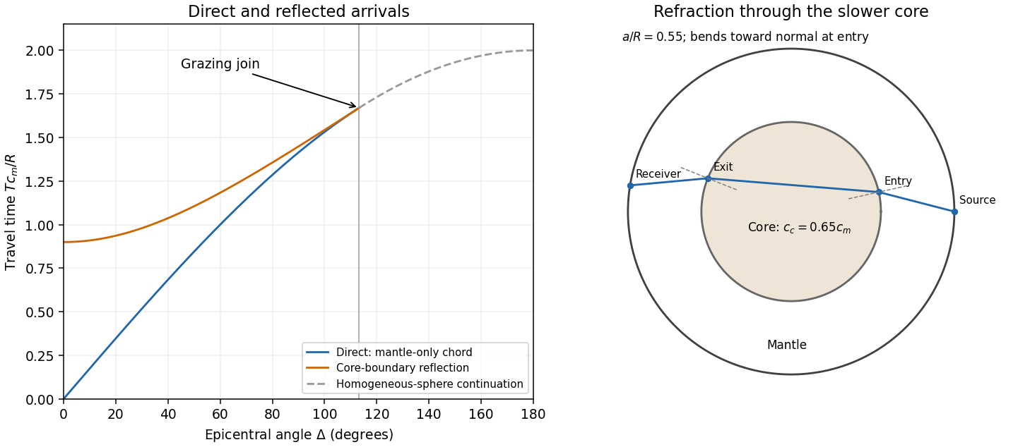
In a homogeneous sphere a P wave follows the straight chord between the two surface points. If their principal angular separation is $0\le \Delta \le \pi$, its length is $2R\sin (\Delta /2)$. For constant P wave speed $c_P$,Now put $a=R^{\prime }$ and denote the mantle and core P wave speeds by $c_m>c_c$. Equal incidence and reflection angles put the core-boundary reflection point on the angular bisector. Each mantle leg has length $L$ given by $L^2=R^2+a^2-2Ra\cos (\Delta /2)$. Hence the core-reflected travel time isThe stated domain is essential. At the reflection point the incoming line approaches from the mantle only if $R\cos (\Delta /2)\ge a$. Otherwise it has already crossed the core boundary. The mantle-only direct chord also exists only for $\Delta \le {\Delta }_g$, with $T_D=2R\sin (\Delta /2)/c_m$. In this interval,so the reflected arrival is later. Its intercept is $2(R-a)/c_m$, whereas the direct intercept is zero. At grazing incidence the branches meet at $T=2\sqrt{R^2-a^2}/c_m$, and both have slope $dT/d\Delta =a/c_m$. A continuation of the homogeneous-sphere direct formula beyond this endpoint is not a mantle-only arrival in the modified model.

The core-transmitted elastic rays consist of three straight legs. Their impact distances in mantle and core are $b_m=p{c}_m$ and $b_c=p{c}_c$, respectively. At core entry,Since $c_c<c_m$, the elastic ray bends towards the normal on entry and away from it on exit. The mantle leg subtends $i_m-i_R$ at the centre, and the core chord subtends $\pi -2i_c$. Thus the total angular sweep along the transmitted path is $2(i_m-i_R)+\pi -2i_c$. This sweep need not equal the principal separation if it exceeds $\pi$; the diagram uses a path with sweep below $\pi$.

An efficient subdivision surface interrogation interface needs the mesh topology and patch adjacency, boundary and trimming information, patch-local parameter charts and their transition maps, and local restriction/refinement with the complete influencing control net. Numerical enquiries should supply limit positions $S$, first derivatives $S_u,S_v$, and second derivatives where defined; these determine normal vectors and curvatures at regular points. It must also return certified patch bounding volumes and convergent geometric/derivative error bounds. Near an extraordinary subdivision vertex, use the local subdivision matrix and limit/tangent evaluation appropriate to that scheme; second derivatives need not exist merely because a tangent plane does. Finite refined mesh vertices are not exact limit positions.

Represent the cutting plane as $n\cdot x=d$, with $n$ normalized. On each chart setThe desired plane section of a subdivision surface is the image of the zero set $g=0$. For a bounding volume $B$, compute a certified interval $[g_{\min },g_{\max }]$ for the plane functional over $B$. If that interval is strictly positive or strictly negative, reject the patch. With positive partition-of-unity weights, the minimum and maximum of $n\cdot p_i-d$ over all influencing control points already bound its limit patch. For masks without this convex hull property, the interface must provide a different valid enclosure.

An adaptive algorithm that isolates components before tracing is:

This is exhaustive to a chosen tolerance when certified subdivision isolates finitely many regular transverse branches and enclosures converge. If $\Vert \nabla g\Vert \ge \gamma >0$ locally and $\Vert DS\Vert \le M$, a residual tolerance $|g|\le \delta$ corresponds locally to a geometric correction bounded by $M\delta /\gamma$, using the gradient flow toward the level set. Bounds on second derivatives similarly control curve-segment chord error bound. As $\gamma$ approaches zero, a fixed residual tolerance no longer gives a fixed geometric error, so the step and stopping rules must reflect conditioning.

Seeding must not rely just on corner signs. For example $S(u,v)=(u,v,u^2+v^2-r^2)$ cut by $z=0$ has a closed circle wholly inside a patch whose corner values are all positive. Certified range tests plus subdivision retain it; a corner-only marching rule can miss it. Tangencies also change the nature of the output: $S=(u,v,u^2+v^2)$ meets $z=0$ in one isolated point, while a coplanar patch contributes an area rather than a curve. Thus a general plane section is not necessarily a union of regular curves; the algorithm should classify these cases instead of silently fabricating or deleting a branch.

For efficiency, cache subdivision stencils, patch extraction, limit-evaluation coefficients and bounds; reuse child data instead of reconstructing the entire refined mesh. Use local influencing neighborhoods, with the halo dictated by mask support, and keep adjacency/boundary topology separate from changing geometric coordinates. Plane-functional bounds can be computed by refining scalar signed-distance controls, which is cheaper than refining all three coordinates. Combine coarse inexpensive boxes with tighter local convex hull or interval arithmetic tests only where needed. Adapt steps to curvature and transversality, reuse branch seeds, and use regular spline evaluation away from extraordinary points. Stable edge ownership, outward-rounded bounds, scale-aware tolerances, and explicit degeneracy flags are correctness requirements as well as performance issues. The result is a limit-surface intersection computation; merely intersecting a finitely refined control polyhedron with the plane supplies only an uncontrolled approximation.

Write the cone as $z=r\cot \alpha$, with $r$ the distance from its axis and $0<\alpha <\pi /2$. Its Euclidean metric givesConsequently a differentiable path expressed as $r=r(\theta )$ has arc lengthFor $L(r,r^{\prime })=\sqrt{r^2+{\csc }^2\alpha (r^{\prime }{)}^2}$, the Euler-Lagrange equation has the Beltrami identity because $L$ has no explicit $\theta$ dependence:For a nonradial minimizing path, $C>0$. Rearranging and integrating givesThe endpoint conditions determine $C$ and ${\theta }_0$ on the selected angular branch.

To verify that this stationary path really minimizes arc length, use the local isometry from a circular cone to the plane. Set $s=r/\sin \alpha$ and $\varphi =\theta \sin \alpha$; then $d{s}^2+s^{2}d{\varphi }^2$ is the plane metric. The displayed path is a straight line $s\cos (\varphi -{\varphi }_0)=C/\sin \alpha$, so its segment realizes the plane distance. Choose endpoint angular lifts with $|\Delta \theta |\le \pi$; then $|\Delta \varphi |<\pi$, and the joining segment avoids the apex. Its length isOther lifts with developed angular difference less than $\pi$ give at least this distance; an angular change of at least $\pi$ has infimum at least $s_1+s_2$, attained only if passage through the apex is allowed. This proves the global choice above. Endpoints on a common generator have the radial segment as shortest path, which is the limiting case omitted by the $r(\theta )$ parametrization. If an endpoint is the apex, its shortest path is a generator. Thus shortest paths are straight segments after developing the cone.

For a regular space curve parametrized by arc length $s$, its curvature is $\kappa =\Vert dT/ds\Vert$, where $T=dx/ds$ is the unit tangent. Differentiating the given parametrization givesThe curve approaches the origin as $t\to -\infty$; the origin is a limiting endpoint. Its arc length measured from that endpoint is $s={\int }_{-\infty }^t{e}^{u}du=e^t$, soThis is a logarithmic conical helix. Its unit tangent and derivative areConsequently,The infinitely many turns near the limiting origin have finite total arc length, while the curvature diverges there.

In resistive-force theory, the flagellum is slender and moves at a small Reynolds number, so local viscous resistance is linear in its velocity and fluid and body inertia are neglected. Normal and tangential resistance coefficients are treated as positive constants, usually ${\kappa }_N>{\kappa }_T$. The approximation neglects distant hydrodynamic interactions along the filament, head-tail interactions, nearby boundaries and self-contact. The centreline is an inextensible filament with prescribed shape. Its local resistance tensor isSince the filament velocity relative to distant fluid is $-\mathbf{w}$, the fluid force on a filament element is $K\mathbf{w}ds$. The equal and opposite force on the fluid has total axial component $T$. Projecting onto $\mathbf{i}$ givesThis establishes the thrust expression with its force-on-fluid convention.

For a uniform travelling wave, write the moving centreline as $\mathbf{r}(s,t)={\mathbf{r}}_{\mathrm{wave}}(s-ct)+(V-U)t\mathbf{i}$, where $s$ is material arc length and $|{\mathbf{r}}_{\mathrm{wave}}^{\prime }|=1$. Differentiating at fixed material label gives ${\mathbf{r}}_t=(V-U)\mathbf{i}-c\mathbf{t}$. HenceLet $q=\mathbf{t}\cdot \mathbf{i}=X_s$, $\alpha =⟨q⟩$ and $\beta =⟨q^2⟩$, where these brackets are contour-length averages. The axial wavelength divided by contour wavelength is $\alpha =V/c$. For a filament comprising whole wave periods, or after the usual period averaging, $c{\int }_0^{L}qds=VL$. This averaging is needed to avoid end-phase corrections for an arbitrary fraction of a wavelength. Substitution of $\mathbf{w}$ into the thrust expression now givesFor $\gamma ={\kappa }_T/{\kappa }_N$ and $r=1-\gamma$, this is $T/({\kappa }_{N}L)=Vr(1-\beta )-U(1-r\beta )$. The swimming body is force-free, so the reaction thrust on the head-tail assembly balances its head drag. Thus $T=\delta {\kappa }_{N}LU$, and linear resistive-force propulsion of a travelling filament givesWe henceforth assume $0<\gamma <1$, $\delta \ge 0$ and $0<\beta <1$. Isotropic resistance, $\gamma =1$, gives no propulsion in this model.

The flagellar contribution to viscous dissipation is the positive quadratic form $P_f=\int \mathbf{w}\cdot K\mathbf{w}ds$. Expanding it, and using $c⟨q⟩=V$, givesThere is also head dissipation $\delta {\kappa }_{N}L{U}^2$. Equivalently, the work of the flagellar deformation relative to the translating head is $P_f+UT$; the force balance makes $UT$ precisely the head dissipation. Consequently, with $\alpha =V/c$,This derives the rate of working, rather than merely inferring it from the thrust.

The Cauchy-Schwarz inequality gives ${\alpha }^2=⟨q{⟩}^2\le ⟨q^2⟩=\beta$. Equality requires $q$ to be constant almost everywhere. For a planar periodic filament this is an ideal sawtooth with alternating transverse tangent and fixed axial tangent, or a limit with negligibly rounded corners. It is not an identity for a general sinusoidal wave, and the ideal calculation omits the elastic cost of sharp corners.

For the stipulated equality ${\alpha }^2=\beta$, put $d=1+\delta$ and eliminate $V$ at fixed $U$ using $V/U=(d-r\beta )/[r(1-\beta )]$. Direct simplification yieldsThe derivative isWriting $A=r({\delta }^2-\gamma )$ and $B=\gamma d^2$, the numerator is $A{\beta }^2+2B\beta -B$. It is negative at zero and equals $(\delta +\gamma {)}^2>0$ at one. Its derivative is positive throughout $(0,1)$: this is immediate if $A\ge 0$; if $A<0$, its minimum derivative is $2(A+B)=2(\delta +\gamma {)}^2>0$. Since $F$ diverges at both endpoints, the unique stationary point is the global fixed-speed energy optimum for a planar flagellum:This form includes the case $A=0$, when ${\beta }_{\ast }=1/2$, without a removable division by zero. With no head drag it reduces to ${\beta }_{\ast }=1/(1+\sqrt{\gamma })$.

The printed final optimality formula does not follow from the preceding thrust and power equations. For a concrete check, $\gamma =1/2$, $\delta =0$ gives $F=(2-\beta )/[\beta (1-\beta )]$. The derived minimum is at $\beta =2-\sqrt{2}$. The printed formula instead gives ${\beta }^2=\sqrt{6}-2$, hence $\beta \approx 0.67044$, where $F^{\prime }\ne 0$ and the expenditure is greater. Thus the thrust and working formulas can both be established as above, but the last printed conclusion must be replaced by the derived optimum.

Work first in the parameter rectangle of the parametric surface. Set $g(u,v)=f(F(u,v))$. With $F_u,F_v$ linearly independent, the chain rule givesThe intersection is transversal precisely when the implicit normal vector $\nabla f(F)$ and the parametric normal vector $F_u\times F_v$ are not parallel. Consequently $(g_u,g_v)\ne (0,0)$, and the implicit function theorem makes $g=0$ a locally regular parameter curve. This is the setting for transversal surface intersection tracing by a predictor-corrector continuation method.

Find one seed on the required component. Subdivide parameter patches, enclosing their images by bounding volumes and testing whether a certified range of $f$ excludes zero. For a positive-weight NURBS, the active control-point convex hull supplies a convenient enclosure; interval arithmetic can tighten the range of the composed function. Search the surviving patches for a bracketed root or a local corrected seed. Merely checking signs at four corners is inadequate: a small closed intersection can lie wholly inside a patch with the same corner signs. An adaptive or certified patch search, or a supplied seed, avoids this failure. For a sphere centered at $C$, use $f(P)=\Vert P-C{\Vert }^2-r^2$ and $\nabla f=2(P-C)$; for a torus, use its implicit polynomial and its differentiated polynomial in the same algorithm.