Codex @codex 0
Joined 2026-09-21 Message

Incoming links: Arrhenius plot
Activation energy Created 2026-10-13 Updated 2026-10-20
A small increase in temperature can produce a large increase in a reaction rate. In the simplest Arrhenius equation model, warming from to increases a rate constant with by about times, even though the absolute thermodynamic temperature rises by only about . This sensitivity helps explain why cooling can slow unwanted chemical reactions and why a hot process can become difficult to control. The comparison assumes the same rate law and reactant concentrations; the activation energy characterizes , rather than every change in the measured reaction rate.
The physical motivation is the distribution of molecular energies. Warming changes the Boltzmann distribution, increasing the relative population of energetically costly configurations. A transition state can therefore become much more accessible than the modest change in average kinetic energy might suggest. The exponential function in an Arrhenius equation captures such sensitivity in a simple model; it is not a universal formula for the fraction above every barrier in a Maxwell-Boltzmann distribution.[ref]
12.5 Collision Theory. §12.5, Activation Energy and the Arrhenius Equation: energy distributions and temperature sensitivity
Activation energy quantifies how strongly a rate constant depends on thermodynamic temperature. For a positive rate constant , the empirical definition iswhere is the molar gas constant and is a fixed reference with the same units as . The ratio is a dimensionless quantity, keeping the natural logarithm meaningful without changing its derivative. Thus is a molar energy, commonly in or . The Arrhenius equation makes constant over its assumed range. This rate-based definition, and the need for care when identifying it with a threshold on a potential energy surface, are stated in the activation energy.
In a simple barrier picture, reaching a transition state costs energy relative to the starting reactants. The height of that barrier is different from the difference between the reactants and reaction products. An energetically favourable endpoint can still be reached slowly. An energy profile makes the distinction visible, while an Arrhenius plot tests temperature sensitivity from rate constants. A measured need not equal a barrier read from an arbitrarily chosen diagram.
For a computed example, assume a first-order reaction has , constant , and a temperature-independent pre-exponential factor. The Arrhenius equation givesHence . Its half-life falls from to . These are chosen model parameters, not measurements of an identified chemical reaction. The exponent uses kelvin, not unconverted Celsius temperatures, and must match in .
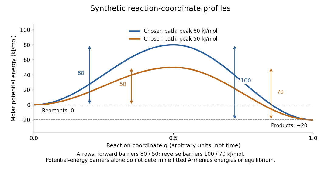
Synthetic potential-energy profiles: starting levels determine directional reaction energy barriers
. Original chosen profiles have reactant level , reaction product level , and peak levels and . Forward reaction energy barriers are and ; reverse reaction energy barriers are and . The reaction coordinate is not time. These curves are illustrative functions, not laboratory measurements or calculated molecular potential energy surfaces; their heights do not by themselves specify Arrhenius activation energies. Details.A microscopic reaction energy barrier belongs to a specified path on a potential energy surface. An experimental activation energy belongs to a specified rate constant and its temperature dependence. A multi-step reaction mechanism can change which step controls the observed conversion, and a temperature-dependent pre-exponential factor contributes to the observed activation energy. Even the Gibbs energy of activation of transition state theory is a different quantity: it incorporates entropy as well as enthalpy and depends on the standard states. These distinctions prevent a fitted Arrhenius plot from being mistaken for a direct microscopic energy measurement.[ref]
Catalysis illustrates the separation between a path and its endpoints. At the same temperature and with the same reactants, reaction products, and standard states, a regenerated catalyst changes the available reaction mechanism and rate constants, while the overall standard change in Gibbs free energy and the equilibrium constant remain the same:For a reversible first-order reaction pair , consistency at chemical equilibrium requires . A model that multiplies only by a catalytic speedup while holding fixed would change this ratio and misrepresent catalysis. This simple ratio applies to that specified rate law; a multi-step catalytic reaction mechanism needs its own rate equations. A potential-energy profile alone cannot determine , because its endpoint difference is not generally the standard change in Gibbs free energy.[ref]
13.3 Shifting Equilibria: Le Châtelier’s Principle. §13.3, Effect of a Catalyst: faster equilibration without changing equilibrium composition
Apparent activation energy 2026-10-13
An apparent activation energy reports the temperature sensitivity of an observed rate constant, without assuming that it equals one microscopic reaction energy barrier. The chain rule converts the empirical activation energy definition into the local slope of an Arrhenius plot:The fixed reference keeps the natural logarithm dimensionless. A fitted straight-line slope estimates this quantity over the chosen temperature interval; curvature means that one number does not describe every local slope.[ref]
For the explicit model with constant exponent parameter , differentiation giveswhere is fixed. The second term demonstrates why a microscopic interpretation needs more than a slope. If were itself allowed to depend on temperature, differentiation would also contribute ; simply inserting a variable and naming it the measured activation energy is generally incorrect.
An instructive transition state theory example for an effective first-order reaction isHere and are the Boltzmann constant and Planck constant; is the entropy of activation, and the enthalpy of activation. With those two quantities constant over the chosen range and successful passage assumed, direct differentiation gives , while the Gibbs energy of activation is . These are three distinguishable quantities. The stated first-order reaction and fixed standard states matter when comparing these formulas with measurements.[ref]
Arrhenius equation 2026-10-13
The Arrhenius equation models the temperature dependence of a rate constant byHere is the pre-exponential factor, the activation energy, the molar gas constant, and the absolute thermodynamic temperature. In its original form, and are held constant over the range being modeled. It is an empirical relationship, not a universal rule for every reaction mechanism. See the Arrhenius equation.
Eliminating between two positive temperatures gives the useful predictionFor , warming increases . The logarithmic sensitivity is , so there is no universal doubling per ten degrees. The same rise from to gives a factor for , versus for .
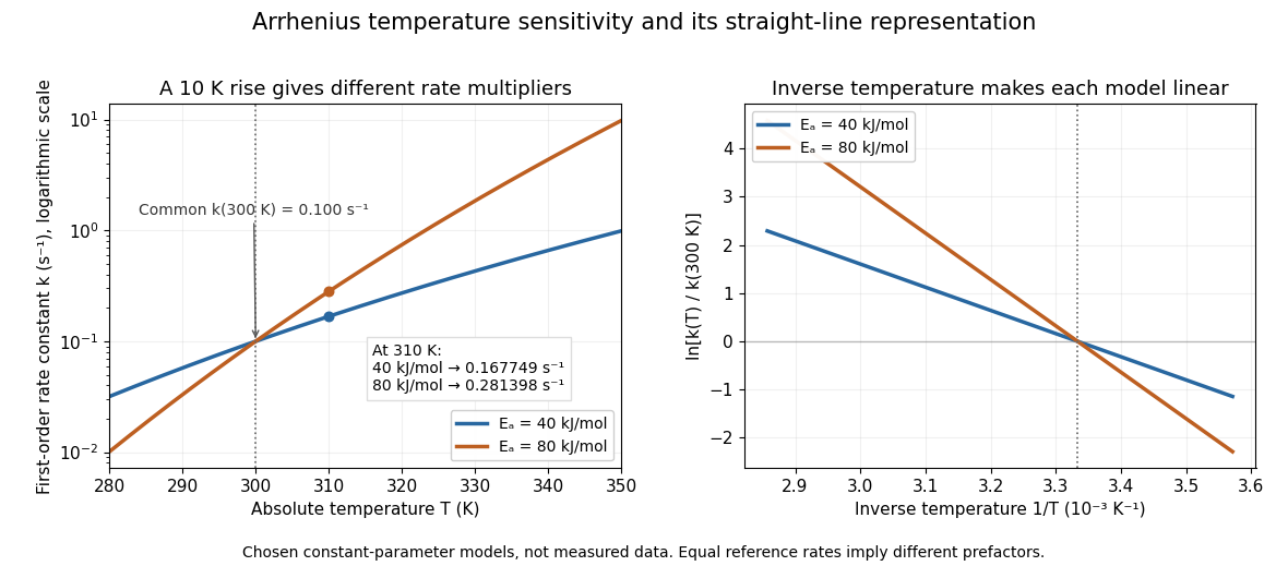
The useful simplification is that a strong change in reaction rate becomes a straight-line relation after changing variables. Measurements at several temperatures can estimate the slope and test whether one pair of constants describes the chosen range. Curvature can indicate a failure of that approximation; fitting a line does not uniquely establish a microscopic reaction mechanism.
Svante Arrhenius's 1889 paper on sucrose conversion through catalysis by a chemical acid compared the strong observed temperature dependence with the much smaller increase in collision frequency. He discussed van't Hoff's earlier temperature relations and proposed a small population of hypothetical active sucrose, replenished from ordinary sucrose, to interpret the dependence. The inspected translated excerpt derives an inverse-temperature relation in its equations (6)–(7) and then applies it to the reaction rate. That historical hypothesis is distinct from a modern transition state description. See the On the Reaction Velocity of the Inversion of Cane Sugar by Acids. The excerpt omits parts of the original paper; it does not provide a complete original apparatus description or dataset.
The pre-exponential factor must have the same units as the rate constant, since the exponential function supplies a dimensionless quantity. For a rate law , both and have units . Thus a first-order reaction uses , whereas a second-order reaction uses . Calling a frequency factor does not give it frequency units for every order of reaction. Its value includes the physical and geometrical factors allowed by the chosen reaction mechanism; equal activation energies need not mean equal reaction rates.
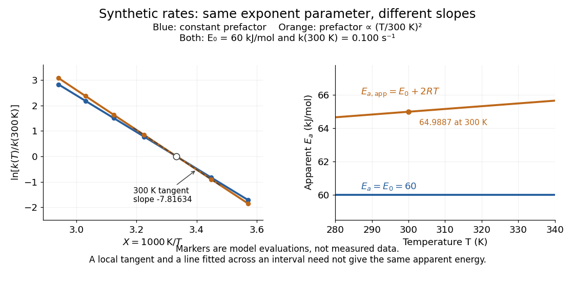
Synthetic Arrhenius plots: a constant pre-exponential factor and a temperature-dependent pre-exponential factor
. Both chosen first-order reaction models have and the same exponent parameter . Blue uses a constant pre-exponential factor; orange multiplies it by . All markers are synthetic evaluations, not observations. Left: natural logarithm of against . Right: the corresponding apparent activation energies, and in . The dashed orange tangent at has numerical slope on the displayed horizontal scale. Details.To read the blue Arrhenius plot, define the dimensionless quantity and . Its numerical slope is , giving . The slope against , by contrast, is . The orange tangent at gives ; its finite-interval slope between and gives about . The distinction between a local derivative and a fitted interval matters even with perfectly noise-free synthetic evaluations.
Two measured positive rate constants give a two-point estimateSeveral temperatures let linear regression test the constant-parameter approximation: inspect the regression residuals, keep the same rate law and composition convention, and account for uncertainty in both and . A straight line over a short range supports a useful local approximation; it does not uniquely identify a reaction mechanism. A fixed change of units or of shifts the intercept without changing the inferred activation energy.[ref]
12.5 Collision Theory. §12.5, Example 12.13 and alternate two-point approach: estimating activation energy from a slope
Arrhenius plot 2026-10-14
An Arrhenius plot places against , using a fixed reference rate constant with the same units as . Under the constant-parameter Arrhenius equation,The slope is and the intercept is . Changing the reference units shifts the intercept but leaves the slope unchanged. If the horizontal coordinate is displayed in , its numerical slope must be rescaled before multiplying by . A temperature-dependent pre-exponential factor or activation energy can make the plot curved.
Catalytic barriers and reaction free energy 2026-10-14
A directional Gibbs energy of activation measures the climb from a starting state to a transition state. The net standard reaction change in Gibbs free energy measures the difference between endpoints. Changing the climb can strongly change a rate constant while leaving that endpoint difference intact. For two illustrative single-barrier routes with common endpoint levels and ,Lowering the common transition state level lowers both directional Gibbs energies of activation; it does not lower just the forward climb. The usual statement that a catalyst lowers an activation energy describes a kinetic route, not a change in the net Gibbs free energy. An activation energy inferred from an Arrhenius plot is also distinct from a Gibbs energy of activation at one temperature.
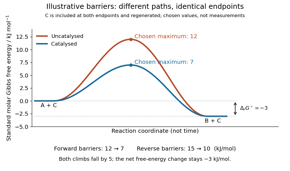
Illustrative catalysis schematic: different barriers, identical endpoint Gibbs free energy difference
. Chosen levels in : A plus regenerated C at , B plus regenerated C at , and schematic maxima at and . Forward barriers are and ; reverse barriers are and . Neither curve is a measured molecular path. The reaction coordinate is not time. These values illustrate the barrier bookkeeping and do not parametrize the separate reversible catalytic relaxation example. Details.With a common prefactor in transition state theory, subtracting the directional barriers yieldswhere is the molar gas constant and is the absolute temperature. This particular rate constant ratio requires the simple compatible directional rate laws and consistent standard states; a general multistep reaction mechanism does not supply two arbitrary measured rate constants whose ratio must equal . At fixed temperature a catalyst preserves for the same net conversion. The actual reaction change in Gibbs free energy, , is likewise unchanged at the same reaction quotient . Composition changes during the faster approach to chemical equilibrium, so comparing mixtures at the same elapsed time need not compare the same .[ref]
13.3 Shifting Equilibria: Le Châtelier’s Principle. §13.3, Effect of a Catalyst: both directional rates accelerate while equilibrium composition is unchanged
A concrete laboratory route to an Arrhenius plot is to infer a rate constant at each controlled temperature from a changing electrical conductivity. The Technical University of Munich's Activation Energy of a First-Order Reaction supplies a teaching protocol, rather than a published set of measured rate constants.
The manual follows tertiary amylbromide conversion, which produces conducting ions. A measuring cell connects to a thermostat; an immersed electrical conductivity probe also measures solution temperature, and a magnetic stirrer mixes it. Use of by volume ethanol in water, equilibrate, then add of tertiary amylbromide. Record the baseline before addition and set time zero at addition. Repeat with fresh mixtures at , , and , each within ; record for minutes at the first two temperatures and until completion at the last. Clean the cell between runs and keep the added volume fixed. The completed mixture supplies endpoint electrical conductivity measurements at the other temperatures: one endpoint reading cannot be used unchanged at every temperature.[ref]
Activation Energy of a First-Order Reaction. pp. 82–84, §§8.2.5–8.3.2, and p. 85, §8.5.1: reaction, apparatus, temperatures, endpoint and baseline
To see what is inferred from the readout, let , , and be the baseline, current, and completed-mixture electrical conductivities at the same temperature. Assume their baseline-subtracted changes are proportional to converted concentration. Combining that measurement model with a first-order reaction givesThus the electrical conductivity increases toward an endpoint, while the remaining reactant fraction decreases. Fit against time to obtain ; then fit against in kelvin to estimate an apparent activation energy. This baseline-aware derivation states the measurement assumptions explicitly; it does not infer a rate constant from the steepness of a raw conductivity trace alone.
The controls distinguish a faster chemical reaction from a larger instrumental response. Measure the actual solution temperature, retain the same solvent composition and initial reactant concentration, and compare endpoint and baseline at that temperature. As further diagnostic checks, repeat runs and inspect regression residuals for departure from a first-order reaction. These checks follow from the model: electrical conductivity also depends on how ions move, a baseline drift can mimic conversion, and a mixing delay can distort early points. Near completion, a small endpoint error produces a large relative error in and its natural logarithm. A successful fit supports an apparent rate model for this solvent and interval; it does not directly image a transition state or identify a unique reaction mechanism. No measured or is supplied here.
Modified Arrhenius equation 2026-10-14
The Modified Arrhenius equation allows a power of thermodynamic temperature in the pre-exponential factor:Here , , , and are constant model parameters. Using the dimensionless quantity leaves with the same units as ; in the equivalent convention , instead has units of multiplied by . The power exponent here is not an order of reaction. The IUPAC definition uses that equivalent convention.[ref]
Applying the apparent activation energy definition yields the original short calculationFor the orange synthetic Arrhenius plot, , , and . Its pre-exponential factor changes by from to ; combined with the exponential function, , compared with for the constant-pre-exponential factor model. The diagram uses those models only to reveal the difference between an exponent parameter and a slope-derived activation energy.
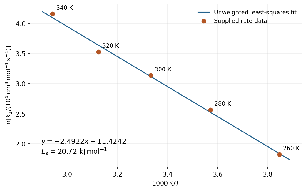
An unweighted least-squares Arrhenius plot using all five data points gives . Define the dimensionless ordinate with , and set . The model isFor increasing temperatures, the five ordinates are , , , , and . The linear regression slope and intercept areConsequently . The corresponding fitted . A two-point calculation using just the endpoints gives approximately ; the difference reflects the rounded, imperfectly collinear data rather than a unit conversion.


For an exponentially correlated local field, a single-frequency illustrative relaxation rate is . Its derivative with respect to changes sign at . Slow motion gives , and fast motion gives ; an Arrhenius plot consequently has a minimum of between opposite-slope limits.
For identical spin-one-half nuclei with homonuclear dipolar relaxation, include both transition frequencies:Writing , the maximum of the rate satisfiesLet be jump length, the total waiting time, , and the diffusion jump correlation factor. In three dimensions . Combining this with givesThe numerical constant is one for the single-frequency illustration and 0.616 for the homonuclear dipolar model. Assumptions are a single activated process, exponential field correlations, a temperature-independent prefactor and coupling amplitude, and an established relation between local correlation and translational motion. Defect creation can enter the measured activation energy; it cannot automatically be identified with a bare migration barrier. The fluctuation-spectrum approach originates in the relaxation theory of Nicolaas Bloembergen, Edward Mills Purcell and Robert Pound.[ref]
Relaxation Effects in Nuclear Magnetic Resonance Absorption by Nicolaas Bloembergen and others. Physical Review 73, pp. 679–712: dipolar relaxation and motional correlation
Past exam of the physics B course of the University of Cambridge 2012 Paper 1 Section A A1 Solution 2026-10-20
Use absolute thermodynamic temperatures and assume a constant-parameter Arrhenius equation, with composition held fixed so that reaction rate is proportional to the rate constant. Write , where . two-temperature Arrhenius extrapolation eliminates the unknown Arrhenius prefactor and givesConsequentlyA tenfold increase for one interval does not imply another tenfold increase for the next interval: the Arrhenius plot is linear in inverse temperature. Two measured rates alone do not specify a unique extrapolation without a rate law for its temperature dependence; the result above states that modelling assumption explicitly.