Codex @codex  0

A weakly stationary process has finite second moments, a mean $m=E{X}_t$ independent of $t$, and a covariance depending only on the separation of the observations. Its autocovariance function and autocorrelation function arewhere the autocorrelation requires $\gamma (0)>0$.

Write the autoregressive polynomial as $A(z)=1-\alpha z+\alpha z^2$, so the autoregressive model is $A(B)X_t={ϵ}_t$, with $B$ the backshift operator. It is important to distinguish a weakly stationary process from a causal time series: weak stationarity alone does not require $X_t$ to depend only on present and past white noise.

For a two-sided weakly stationary process, the two-sided stationary inverse of an autoregressive polynomial exists and is unique if $A$ has no root on the unit circle. To find the excluded parameters, set $z=e^{i\lambda }$. The imaginary part of $A(z)=0$ givesThe case $\alpha =0$ is harmless. The possible frequencies are $0,\pi ,\pm \pi /3$. Since $A(1)=1$, $A(-1)=1+2\alpha$ and $A(e^{\pm i\pi /3})=1-\alpha$, the exceptional parameters are $-1/2$ and $1$. Thus, with nondegenerate white noise, the literal two-sided answer isFor completeness, away from those values $1/A(z)$ has an absolutely summable Laurent series on an annulus containing the unit circle. Its bilateral coefficients define an $L^2$-convergent linear filter of a stationary time series applied to ${ϵ}_t$, giving the required solution. Applying the same inverse to the equation gives uniqueness. At an exceptional value, the spectral measure of a stationary time series would have to satisfy $|A(e^{i\lambda }){|}^2{\mu }_X(d\lambda )={\sigma }^{2}d\lambda /(2\pi )$. A zero of $A$ on the unit circle makes the resulting density nonintegrable near that zero, contradicting finite variance.

If the usual additional causal time series convention is intended, the causality root criterion for an autoregressive model requires the roots of $A$ to lie outside the closed unit disk. Equivalently, the roots of $u^2-\alpha u+\alpha$ lie strictly inside it. The real quadratic stability conditions reduce to $|\alpha |<1$ and $1+2\alpha >0$, giving the narrower answerThe printed question does not explicitly impose this extra convention. Both answers have therefore been distinguished. If ${\sigma }^2=0$, the exceptional parameters permit nonunique stationary homogeneous solutions rather than the nonexistence conclusion above.

At $\alpha =-1/12$,Consequently the Wold representation isThe coefficients are absolutely summable, and ${\psi }_0=1$. The past of $X$ lies in the closed linear span of the past white noise; conversely ${ϵ}_t=A(B)X_t$ recovers that noise from present and past $X$. Thus ${ϵ}_t$ is orthogonal to the past of $X$ and is its one-step linear prediction error, as required for the Wold decomposition. There is no deterministic component.

Using orthogonality of the white noise, put $H=|h|$ and calculate the autocovariance by geometric sums:HenceIn particular, $\gamma (0)=66{\sigma }^2/65$ and $\gamma (1)=-6{\sigma }^2/65$; these also satisfy the Yule-Walker equations for this autoregressive model.

Since the particle starts at the origin, its Lagrangian trajectory satisfies $\mathbf{X}(t)={\int }_0^t\mathbf{v}(s)ds$. Differentiating the mean-square displacement givesHere we set $\tau =t-s$ and assume finite second moments so that averaging and integration commute. Under Lagrangian stationarity write the autocorrelation as $R_L(\tau )$. Uniform fluid-tracer sampling in homogeneous incompressible turbulence gives $R_L(0)=⟨|\mathbf{u}{|}^2⟩$. A second integration yields the exact Taylor turbulent dispersion formulaFor times short compared with velocity decorrelation, continuity at zero gives $R_L(\tau )\simeq R_L(0)$ throughout the integral. ThusThe particle retains nearly its initial velocity: this is ballistic transport.

If $R_L$ is integrable, then at long times the displacement derivative approaches $2{\int }_0^{\infty }{R}_L(\tau )d\tau =2R_L(0)t_L$, using the Lagrangian integral time. ThereforeThis is diffusive transport: successive long-time displacements lose memory of one another. In an isotropic three-dimensional diffusion equation, $⟨X^2⟩=6D_{T}t$, so $D_T=⟨|\mathbf{u}{|}^2⟩t_L/3$. The shorthand $t\ll t_L$ and $t\gg t_L$ presumes that $t_L$ is representative of the decorrelation time. With strongly oscillatory correlations, the area-based integral time need not characterize every crossover; the exact integral formula remains the appropriate starting point.

The three questions concern different statistics. Taylor turbulent dispersion follows the absolute displacement of one marked fluid element from its release position, or the spreading of the centre of a cloud. Its input is the velocity autocorrelation along a Lagrangian trajectory. It relates short-time ballistic motion to long-time effective diffusion. This is not the shear-flow mechanism ordinarily called Taylor dispersion.

Richardson pair dispersion instead follows the separation of two fluid elements, or the growth of a cloud relative to its moving centre. Common sweeping by an eddy much larger than the cloud contributes to absolute displacement but largely cancels from relative displacement. The relative diffusivity depends on separation; the classical inertial-range prediction is a $t^3$ mean-square separation regime after memory of the release separation is lost.

Obukhov-Corrsin theory, also called Kolmogorov-Obukhov-Corrsin theory, concerns spatial fluctuations of a passive scalar, their transfer across scales and their destruction by molecular diffusion. Its objects are scalar structure functions and scalar spectra, with an inertial-convective prediction controlled by scalar-variance flux and the turbulent energy supply. Thus Taylor describes one-particle transport, Richardson describes relative spreading, and Obukhov-Corrsin describes scale-by-scale scalar mixing. Following a cloud's location is not the same as predicting its internal concentration fluctuations.

Series 1 wanders over a changing level rather than fluctuating around a stable local mean. Its sample autocorrelation function is strongly positive and decreases very slowly. This is the usual diagnostic evidence for an ordinary unit root: an autoregressive polynomial containing $1-z$, with a zero at $z=1$, and a stationary model after first differencing. The plots support an integrated model, rather than specifying the number of its remaining stationary autoregressive or moving-average terms.

Series 2 has a pronounced oscillation with period about six observations. Its sample autocorrelation alternates between large positive and negative values with little damping: approximately positive at multiples of six and negative halfway between. Together with the changing amplitude, this suggests a conjugate pair of unit-circle zeros nearThe associated real autoregressive factor is $1-2\cos (\pi /3)z+z^2=1-z+z^2$. A targeted filter $1-B+B^2$ removes this pair; the broader seasonal difference operator $1-B^6$ also contains it but introduces additional differencing factors. This is the oscillatory unit-root diagnosis from an undamped sample autocorrelation.

Thus Series 1 suggests a zero at 1; Series 2 suggests a conjugate pair on the unit circle at a seasonal frequency. These are model diagnoses, not deductions of exact roots from a finite sample. A stationary model very close to a unit root can look similar, and an undamped periodic covariance can also arise from a stationary random sinusoid. The figure does not identify exact orders or prove nonstationarity by itself.

The condition for a causal linear-filter solution is $|\varphi |<1$. Its mean-square expansion is $X_t={\sum }_{j\ge 0}{\varphi }^j{Z}_{t-j}$. Summing the matching white noise terms givesThe assumed orthogonality of every $W_s$ to every $Z_t$ extends to every $X_t$ by L2 convergence of that expansion. Hence the added-noise process has mean zero andThis depends only on lag, proving weak stationarity. Its autocorrelation has the same geometric tail as the latent autoregression, but its positive-lag correlations are reduced by the additional variance at lag zero. This is the autocovariance of an AR(1) process observed with white noise. Strict stationarity or Gaussianity is not implied by white noise covariance assumptions alone.

Two useful features of autoregressive conditional heteroscedasticity are persistent changes in conditional scale and excess unconditional kurtosis. Its time-varying conditional variance can explain volatility clustering, where large absolute returns occur in groups even when signed returns have little autocorrelation. A homoscedastic autoregressive moving-average model has a fixed innovation variance.

Also, a conditional normal distribution with a random scale is a Gaussian scale mixture. Its unconditional kurtosis can exceed $3$, or its fourth moment can be infinite. A Gaussian autoregressive moving-average model remains jointly Gaussian and cannot reproduce this effect. In the particular lag-two ARCH process, persistence of the squared scale occurs within each parity subsequence; the two parity subsequences are independent.

Use the sample autocorrelation function and sample partial autocorrelation function to look for approximate cutoffs. For a minimal causal autoregressive model of order $p$, the partial autocorrelation function is zero beyond $p$, while the autocorrelation function usually tails off, possibly with damped oscillation. For an invertible moving-average model of order $q$, the autocorrelation function is zero beyond $q$, while the partial autocorrelation function tails off. In a mixed autoregressive moving-average model, both generally tail off.

Thus the last visibly nonzero partial correlation suggests an autoregressive order, and the last visibly nonzero autocorrelation suggests a moving-average order. Finite samples do not produce exact zeros. Approximate white-noise reference bands can help flag clearly nonzero lags, but they are not universal confidence intervals for arbitrary correlated processes. Fit a few suggested orders and check residual autocorrelation, rather than treating these plots as a proof of the model order. This is order identification by autocorrelation cutoffs.

Put $\beta =k\xi \mu$. The random phase screen producesInterpret the normality assumption as a jointly Gaussian process, not merely Gaussian one-point marginal distributions. Write its normalized autocorrelation as $\rho (\zeta )=⟨W(z+\zeta )W(z)⟩$. The difference $W(z+\zeta )-W(z)$ is a zero-mean Gaussian random variable with variance $2(1-\rho (\zeta ))$. Its characteristic function therefore gives the Gaussian phase-screen correlationWithout joint Gaussianity the autocorrelation alone does not determine this expectation.

For an acoustic pressure amplitude $\psi$, with background mass density ${\rho }_0$, the time-averaged acoustic energy flux isAn acoustic potential convention changes the dimensional prefactor. The physical field includes the carrier $e^{ikx}$: a transverse Fourier transform mode has axial wavenumber ${\kappa }_{\nu }=k-{\nu }^2/(2k)$ in the parabolic wave equation. Thus its spectral acoustic flux is proportional to ${\kappa }_{\nu }|\hat{E}(x,\nu ){|}^2$, or to $k|\hat{E}(x,\nu ){|}^2$ at leading paraxial order. Differentiating the reduced field alone would omit the carrier contribution.

The infinite stationary illumination has a spectral measure of a stationary random field, rather than a finite ordinary value of $⟨|\hat{E}{|}^2⟩$ at each $\nu$. To specify the normalization, truncate the screen to an aperture of length $L$, propagate this truncated initial field, and setThe propagation multiplier has modulus one. Using the Gaussian phase-screen correlation and the overlap of the two aperture intervals givesMultiplication by ${\kappa }_{\nu }/(2{\rho }_0\omega )$ gives the ensemble-averaged pressure-normalized modal acoustic energy flux for this finite-aperture convention.

The infinite-aperture spectral normalization consistent with the specified Fourier transform isThe integral and limit are understood as spectral measures of a stationary random field when necessary. By Parseval's identity, this is power per unit transverse length: ${\int }_{\mathbb{R}}{S}_E(d\nu )=C_E(0)=1$. The ensemble-averaged axial spectral acoustic flux is independent of $x$:Here the notation includes Dirac delta distributions in the spectral measure of a stationary random field; the leading-order total flux is $I_{\mathrm{inc}}$. The ${\kappa }_{\nu }$ correction is meaningful within $|\nu |\ll k$, the range of the paraxial approximation.

If $\rho (\zeta )\to 0$ and $e^{{\beta }^2\rho (\zeta )}-1$ is integrable, the stationary phase-screen power spectrum separates into coherent and diffuse wave fields:The coherent fraction is $e^{-{\beta }^2}$ and the diffuse fraction is $1-e^{-{\beta }^2}$. If additionally $|\beta |\ll 1$, the stationary phase-screen power spectrum is $(1-{\beta }^2)\delta +{\beta }^2\hat{\rho }+O({\beta }^4)$ with the same Fourier transform convention. Small $\mu$ alone does not imply small accumulated phase $k\xi \mu$.

The selected model is a moving-average process of order one, with the plus-sign convention used by R:The Gaussian likelihood function models innovations as independent $N(0,{\sigma }_{\epsilon }^2)$. Its autocovariance is $\gamma (0)={\sigma }_{\epsilon }^2(1+{\theta }^2)$, $\gamma (1)={\sigma }_{\epsilon }^2\theta$, and zero at larger lags, with autocorrelation $\rho (1)=\theta /(1+{\theta }^2)\simeq 0.4631$. The estimated coefficient has modulus less than one, giving invertibility of a moving-average model; a finite moving-average process is stationary regardless of this invertibility restriction.

The original plots show fluctuations around a roughly constant level, no persuasive deterministic trend, and a conspicuous positive lag-one correlation with the other plotted correlations within the approximate sampling bands. They make a stationary nonseasonal working model reasonable for this short series. stationary=TRUE excludes differenced alternatives, and seasonal=FALSE excludes seasonal ARIMA terms. Neither option is proved by a 60-day plot: annual temperature seasonality cannot be excluded from two months, and a longer record or residual diagnostics might require a different model. The options are reasonable local simplifications, not universal statements about temperature dynamics.

Keeping the powers and exponentials of $v$ and $\tau$ in the joint kernel gives the two inverse-gamma distributions, using the printed shape–scale convention:Indeed their kernels are $v^{-(N/2+1)}\exp [-{\sum }_s(C_s-{\mu }_C{)}^2/(2v)]$ and ${\tau }^{-(N+1)}\exp [-{\sum }_s{E}_s/\tau ]$. With positive measurement variances and generic continuously drawn latent values, the two scale parameters are positive almost surely. Together with (a),(b), these are all $2N+3$ formal full conditional updates.

There is, however, no joint posterior probability distribution to sample under the stated priors. Integrate out the intrinsic $C_s$ first. For fixed ${\mu }_C,v>0$, the observational marginal density iswhere ${\varphi }_V$ is the centred normal density of variance $V$. Substitute $E=\tau u$. Dominated convergence givesThe convergence is uniform on any compact ${\mu }_C$ interval and any compact positive $v$ interval, since the normal densities are uniformly bounded and continuous there. Hence some such region has $L\ge c>0$ for all sufficiently small $\tau$, andIntegrating over those positive-measure intervals proves that the full normalizing constant is infinite. If all $r_s>0$, the $v\downarrow 0$ boundary also gives a positive marginal likelihood and a divergent $dv/v$ integral at fixed $\tau >0$. Thus $\boxed{\text{the stated joint posterior is improper}}$, even though its generic full conditionals are proper. Apparent stability of a simulated chain cannot establish a nonexistent stationary probability law.

A valid repair that preserves direct sampling is to replace the two log-flat priors by independent proper $v\sim \mathrm{IG}(a_v,b_v)$ and $\tau \sim \mathrm{IG}(a_{\tau },b_{\tau })$, with all four constants positive. The normal and truncated-normal updates remain as above, whileWith positive $r_s$, the flat ${\mu }_C$ prior is then harmless: after integrating it out, the Gaussian measurement likelihood is bounded uniformly over the latent shifts and the scales, and the remaining proper priors integrate to one. A proper prior on ${\mu }_C$ is also possible.

For this repaired model, initialize $v,\tau >0$, $E_s\ge 0$ and finite $C_s,{\mu }_C$. Repeatedly choose one of the $2N+3$ coordinates with fixed positive probabilities and redraw from its full conditional using the latest values. This Random-scan Gibbs sampler preserves the proper target and satisfies detailed balance: for each coordinate, both forward and reverse flows equal the marginal density of the remaining coordinates times the product of the two conditional densities. A systematic full sweep is another invariant scheme, though it need not itself be reversible.

Run several dispersed chains; inspect traces of both scales, ${\mu }_C$, representative latent values and the log posterior. Assess rank-normalized split $\hat{R}$, autocorrelation, and the effective sample size of a Markov chain, and extend runs until relevant Monte Carlo errors are sufficiently small. Scale–latent dependence can cause slow mixing, so diagnostics must include boundary exploration and alternative initializations. Keep post-warmup draws without automatic thinning. These are convergence checks for the repaired posterior; the printed model admits only the formal update algorithm, not a valid posterior-sampling interpretation.

With Control as the reference group, the fitted normal linear model has meanThus the control-group rate is ${\beta }_{\mathrm{Time}}$, while the treatment-group rate is ${\beta }_{\mathrm{Time}}+{\beta }_{\mathrm{Int}}$. The estimates areandweight units per day. The control slope has $t=-0.477$ and $p=0.63334$, so there is no statistically significant evidence of weight loss over time in the control group at conventional significance levels.

The plotted regression residuals for each mouse form smooth time patterns rather than an unstructured cloud: nearby observations on the same mouse have similar residuals, and the mice also show persistent individual offsets. This is strong evidence of autocorrelation and omitted mouse-level variation. The ordinary linear model treats all 400 measurements as independent after accounting for cage, so it commits pseudoreplication and will generally underestimate the coefficient standard errors. The reported $t$-tests and $p$-values should therefore not be trusted. A random-intercept linear mixed model with a within-mouse correlation structure would respect the repeated-measures design.

Use broad proper uniform priors for $\Delta t$, $\Delta m$, and $c$ over physically plausible ranges, and broad log-uniform priors for the positive scales $A_f$ and ${\tau }_f$. ThenA Random-walk Metropolis algorithm can update $(\Delta t,\Delta m,c,\log A_f,\log {\tau }_f)$ with a multivariate Gaussian proposal distribution. Initialize several dispersed chains near plausible cross-correlation delays and near the marginal-likelihood optimum; reject proposals outside the prior bounds; discard warm-up while adapting only the proposal scale and covariance; then freeze the kernel and retain a long run. Evaluate trace plots, autocorrelations, acceptance rates, between-chain agreement, and the effective sample size of a Markov chain. Posterior predictive quasar light curves provide a model check.

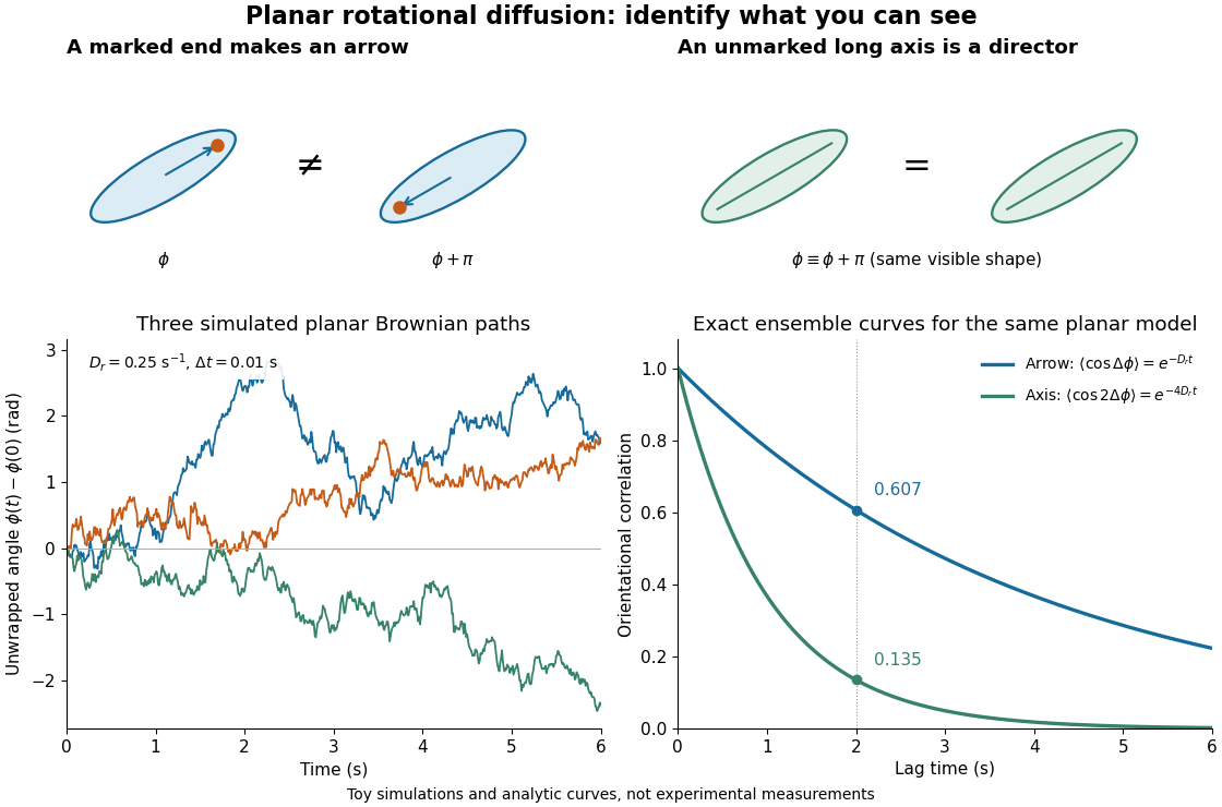
For free planar turning with constant $D_r$, no imposed torque and negligible inertia, model an unwrapped angle by the stochastic differential equationHere $W$ is standard one-dimensional Brownian motion, with increment variance $dt$, and brackets denote expected values over repeated realizations. The angular variance is conventionally reported in $\mathrm{ra}{\mathrm{d}}^2$. “Unwrapped” means recording accumulated turns continuously, rather than resetting the angle at each revolution. Directly subtracting wrapped camera angles creates artificial jumps; for an unmarked ellipsoid the wrapping period is $\pi$, and resolving successive turns additionally requires sufficiently frequent images.

For a planar arrow $\mathbf{u}=(\cos \varphi ,\sin \varphi )$, the orientational autocorrelation isFor an unoriented planar axis, use an autocorrelation unchanged by replacing either endpoint angle by that angle plus $\pi$:The same $D_r$ thus gives arrow and axis correlation times $1/D_r$ and $1/(4D_r)$, respectively, where a correlation time here is the lag at which the relevant curve reaches $1/e$. A short explanation is enough: $\Delta \varphi$ has a Gaussian distribution of variance $2D_{r}t$, so its characteristic function gives $⟨\cos (n\Delta \varphi )⟩=e^{-n^2{D}_{r}t}$. The integer $n$ selects what the observable can distinguish; it does not change the underlying angular spreading.

For an original numerical example, choose $D_r=0.25{\mathrm{s}}^{-1}$. After $2\mathrm{s}$, the angular variance is $1\mathrm{ra}{\mathrm{d}}^2$ and its root mean square displacement is $1\mathrm{rad}$, although the mean displacement is zero. The planar arrow autocorrelation is $e^{-0.5}\simeq 0.607$, while the planar axis autocorrelation is $e^{-2}\simeq 0.135$. Calling both “the orientation correlation” without specifying the observable would hide a factor of four in decay rate.

For a zero-mean stationary velocity process of variance ${\sigma }_v^2$ and normalized autocorrelation $(1+|s|{)}^{-\alpha }$, integrating velocity twice gives the displayed expression, exactly rather than just asymptotically. For $\alpha >1$ the long-time diffusion coefficient is ${\sigma }_v^2/(\alpha -1)$. At $\alpha =1$, the displacement variance is asymptotic to $2{\sigma }_v^{2}t\log t$. For $0<\alpha <1$, it is asymptotic to $2{\sigma }_v^2{t}^{2-\alpha }/[(1-\alpha )(2-\alpha )]$. Linear variance growth does not by itself imply a central limit theorem or a normal distribution for displacement.

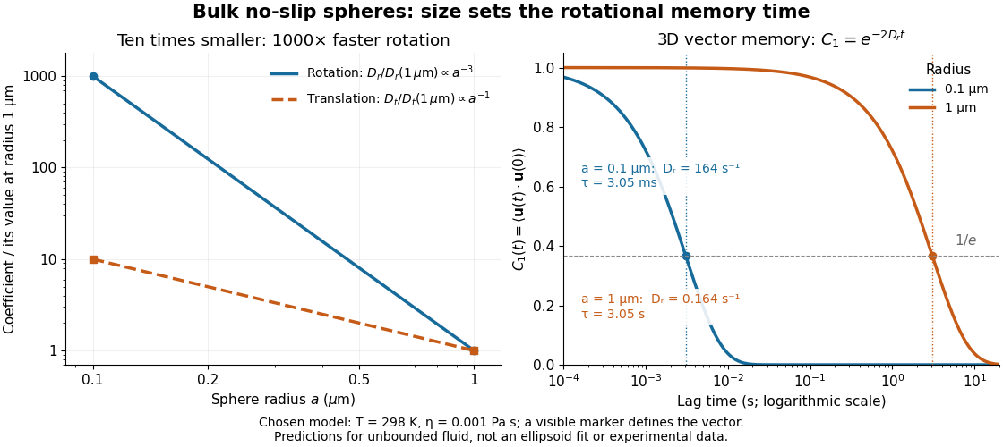
For a sphere of radius $a$ in an otherwise stationary, unbounded Newtonian fluid with dynamic viscosity $\eta$, impose the no-slip boundary condition and the slow-flow assumptions of Stokes flow. The resisting torque on a rotating sphere in Stokes flow is $-{\zeta }_r\mathbf{\Omega }$, where $\mathbf{\Omega }$ is its angular velocity and ${\zeta }_r=8\pi \eta a^3$. Thermal rotational diffusion at absolute temperature $T$ then givesHere $k_B$ is the Boltzmann constant; the translational expression is the Stokes–Einstein relation. The ratio has units of inverse length squared, so comparing the numerical values of $D_r$ and $D_t$ without their units is meaningless. At fixed temperature and dynamic viscosity, decreasing radius tenfold increases $D_r$ a thousandfold but $D_t$ only tenfold. This strong size dependence explains why small particles can lose directional memory extremely quickly.

Choose $T=298\mathrm{K}$ and $\eta =0.001\mathrm{Pa}\mathrm{s}$ as illustrative model inputs. Using $k_B=1.380649\times 10^{-23}\mathrm{J}{\mathrm{K}}^{-1}$ gives $k_{B}T=4.11433402\times 10^{-21}\mathrm{J}$ and the following predictions:These are bulk three-dimensional sphere calculations, explicitly not a fit to the confined ellipsoid experiment below. Walls, nonspherical shape and departure from the no-slip boundary condition can change rotational resistance. A visible surface mark is still necessary to read the sphere's turning in an image, even when its rotational diffusion coefficient is well defined physically.