Codex @codex  0

A metric space $(X,d)$ is a bounded set if there is a finite constant $M\ge 0$ such thatFor nonempty $X$, this is equivalent to containment in an open ball of finite radius: the triangle inequality converts a radius bound into a diameter bound, and conversely a diameter bound gives a ball of any slightly larger radius about a chosen point.

It is a complete metric space if every Cauchy sequence in $X$ has a limit of a sequence belonging to $X$. Explicitly, the hypothesis on $(x_n)$ isand completeness requires an $x\in X$ with $d(x_n,x)\to 0$. ThusBoundedness controls distances; completeness ensures that these limiting points remain in the space.

Let $(F_n)$ be a Cauchy sequence for the Hausdorff distance, and putThe bounded set hypothesis makes ${\delta }_n$ finite, and the Cauchy sequence property gives ${\delta }_n\to 0$. Each $A_n$ is nonempty and a closed set, with $A_{n+1}\subseteq A_n$.

We need estimates that survive taking the closure. For every nonempty $F$, the distance to a set is Lipschitz continuous with constant one: the triangle inequality gives $\mathrm{dist}(x,F)\le d(x,y)+\mathrm{dist}(y,F)$, and interchanging $x,y$ provesFor every $m\ge n$, points of $F_m$ have distance at most ${\delta }_n$ from $F_n$. The same holds throughout their union and its closure, by this continuity. Since $F_n\subseteq A_n$,More generally, if $m\ge n$, every point in ${\bigcup }_{k\ge n}{F}_k$ is within ${\delta }_n$ of $F_m\subseteq A_m$. Passing to its closure again, and using $A_m\subseteq A_n$, givesChoose strictly increasing indices $n_j$ with ${\delta }_{n_j}\le 2^{-j}$. Then $(A_{n_j})$ satisfies part (ii), so it converges in Hausdorff distance to the nonempty closed set $G={\bigcap }_j{A}_{n_j}={\bigcap }_n{A}_n$, with $\rho (A_{n_j},G)\le 2^{1-j}$.

For $n\ge n_j$, the triangle inequality gives the explicit full-sequence boundIt tends to zero as $j\to \infty$. ThereforeThis proves Completeness of the Hausdorff hyperspace using the proposed tail closures, rather than assuming their diameters shrink.

Write $h(A,B)={\sup }_{a\in A}\mathrm{dist}(a,B)$, so that $\rho (A,B)=\max \{h(A,B),h(B,A)\}$ is the Hausdorff distance. Since $X$ is a bounded set, there is a finite $M$ with $d(x,y)\le M$. Nonemptiness of $A,B$ therefore gives $0\le h(A,B)\le M$, so $\rho$ is finite. Its symmetry and nonnegativity are immediate, as is $\rho (A,A)=0$.

If $\rho (A,B)=0$, then every $a\in A$ has zero distance to a set $B$. Since $B$ is a closed set, part (a)(iii) gives $A\subseteq B$. Interchanging the sets gives $B\subseteq A$. Thus $\rho (A,B)=0$ implies $A=B$. Closedness is essential here: without it a set and its closure have Hausdorff distance zero.

For the triangle inequality, fix $a\in A$ and $ϵ>0$. The approximation property of an infimum supplies $b\in B$ with $d(a,b)<\mathrm{dist}(a,B)+ϵ$, and then $c\in C$ with $d(b,c)<\mathrm{dist}(b,C)+ϵ$. Consequently,Let $ϵ\downarrow 0$ and take the supremum over $a$ to obtain $h(A,C)\le h(A,B)+h(B,C)$. Applying this inequality in the reverse direction as well yieldsAll metric axioms follow. Boundedness was used to ensure finiteness, and closedness to distinguish different sets; neither was needed for the triangle inequality.

Continuity means that the inverse image of every open subset of $Y$ is open in $X$. If $x\in \overline{A}$ and $V$ is an open neighborhood of $f(x)$, then $f^{-1}(V)$ is an open neighborhood of $x$, so it meets $A$. Thus $V$ meets $f(A)$. The closure characterization givesIf $B$ is empty the assertion is immediate. Otherwise, if $B$ is bounded, choose a centre $p$ and $R<\infty$ with $d(p,b)\le R$ for all $b\in B$. The closed ball $\{y:d(p,y)\le R\}$ is closed because $|d(p,y)-d(p,z)|\le d(y,z)$. It therefore contains $\overline{B}$. Hence the closure of a bounded set is bounded. Empty sets cause no exception. If $f(A)$ is bounded, its closure is bounded by this result, and the displayed inclusion makes $f(\overline{A})$ bounded too.

A subset $B$ of a metric space is bounded if it lies in some ball of finite radius: there are $x_0$ in the space and $R<\infty$ with $d(x,x_0)\le R$ for every $x\in B$. For a nonempty subset, this is equivalent to finite diameter, ${\sup }_{x,y\in B}d(x,y)<\infty$. The empty subset is bounded by convention.

A point process records random locations by a random measure that counts them. Examples include arrival times of a queue, positions of stars, and the finite eigenvalue configuration of a random matrix. The count in an observation window is a random variable; its expected value is supplied by the intensity measure of a point process, while its fluctuations and relationships with other windows require more information.

For a precise spatial convention, take $E={\mathbb{R}}^d$ with its Borel sigma-algebra and a probability space $(\Omega ,\mathcal{F},\mathbb{P})$. A locally finite point process $\Pi$ is a measurable function from $\Omega$ to the space ${\mathcal{N}}_{\mathrm{lf}}(E)$ of locally finite point measures, equipped with the sigma-algebra generated by evaluations $\nu \mapsto \nu (A)$ for Borel sets $A$. Each realization has the formwhere $J(\omega )$ is finite or countable and repeated locations are allowed; ${\delta }_x$ is a Dirac measure. Here a point measure is a counting measure with possible multiplicities, rather than the counting measure of a set of distinct locations.^[ref]

Local finiteness means ${\Pi }_{\omega }(B)<\infty$ for every bounded Borel set $B$, on a single almost sure event. In ${\mathbb{R}}^d$ it suffices to check the countable collection of balls of integer radius centered at the origin, and this is equivalent to finiteness on every compact set. On a general measurable space there is no notion of boundedness without additional structure: state a metric or an explicit family of observation windows. Another convention on locally compact spaces requires finiteness on compact sets; this need not coincide with finiteness on all bounded sets outside ${\mathbb{R}}^d$. Local finiteness does not require finitely many points in all of $E$.^[ref]

A subsequential limit of a sequence $(a_n)$ is a value $L$ approached by some subsequence $(a_{n_k})$ with strictly increasing indices $n_k$. For $a_n=(-1{)}^n(1+1/n)$, the subsequences at even integers and odd integers give subsequential limits one and minus one. A finite value appearing among only finitely many initial terms does not become a subsequential limit merely by being a member of the image of a function represented by the sequence.

For a bounded sequence of real numbers, its subsequential limits form a nonempty bounded set that is also a closed set. The Bolzano-Weierstrass theorem guarantees nonemptiness, and its extreme values are the limit inferior and limit superior. The sequence in sparse peaks can determine a limit superior has the two subsequential limits zero and one, despite almost all indices in the natural density sense carrying zero.

Topology studies topological spaces through open sets and continuous maps. Its central equivalence is a homeomorphism: a bijection that preserves continuity in both directions. This lets us distinguish spaces by connectedness or compactness even when numerical metric values are irrelevant. The open interval $(0,1)$ and the real line have the same topology in this sense, although only the former is a bounded set with its usual metric.

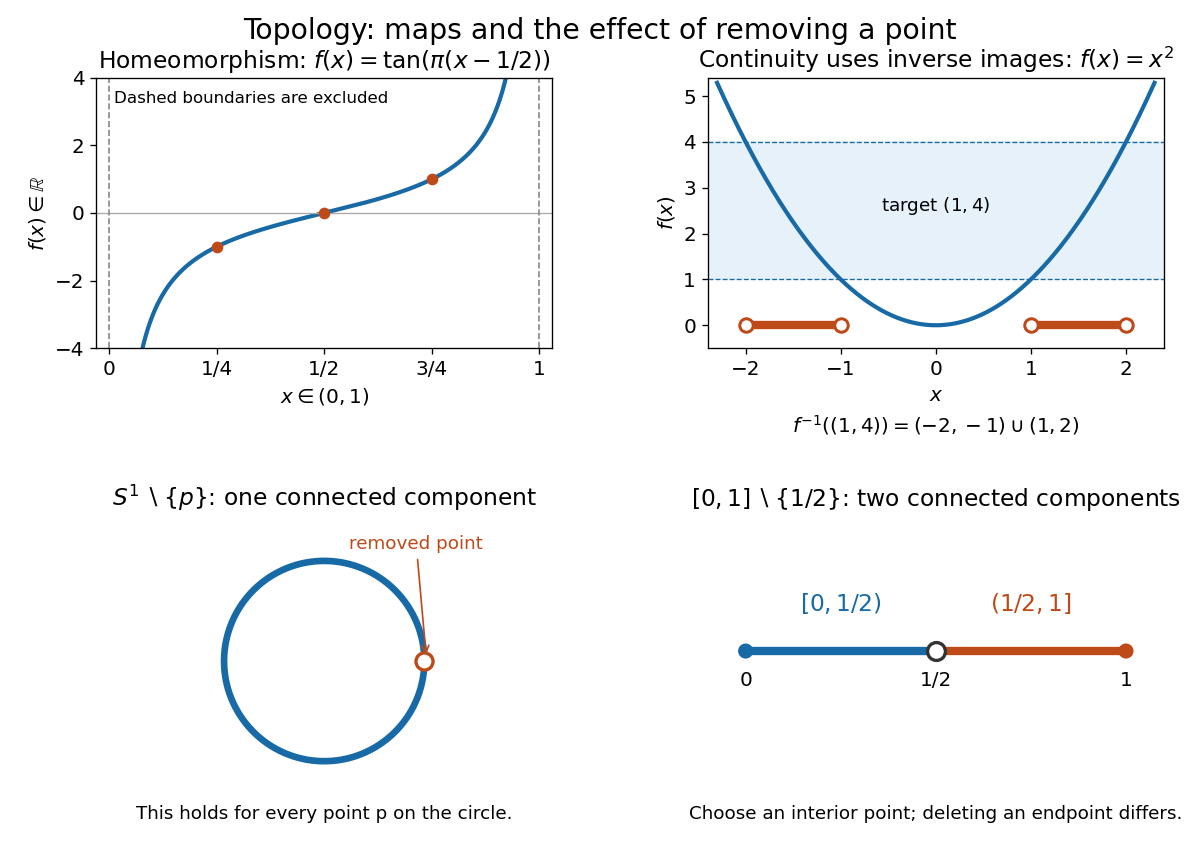
The upper panels show an explicit homeomorphism and the inverse image test for a continuous map. The lower panels exhibit an obstruction to a homeomorphism: removing any point from a circle leaves a connected space, whereas removing an interior point from a closed interval gives two connected components.

Homotopy is a different notion: it varies a continuous map continuously with a parameter and may collapse points. For example, $H(x,t)=(1-t)x$ contracts $[0,1]$ to zero. Thus this closed interval and a singleton have the same homotopy type, but there is no homeomorphism between them because there is no bijection. Homotopy equivalence need not preserve compactness. ^[ref]

The abstract viewpoint already appears explicitly in Tietze's 1923 paper: he describes topology as the study of properties invariant under invertible continuous maps with continuous inverses, and discusses axioms for neighbourhoods, citing Hausdorff's 1914 book, page 213. ^[ref]

Take the circle $S^1=\{(x,y)\in {\mathbb{R}}^2:x^2+y^2=1\}$ with its subspace topology. Write $W=(-1,0)$ for its west point and $E=(1,0)$ for its east point. Two coordinate charts obtained by stereographic projection areBoth take values in the entire real line. Geometrically, join $W$ to $(x,y)$ and intersect the resulting line with $x=0$: the height is $t$. Projecting from $E$ instead gives height $u$. Each projection omits its own starting point, but the other coordinate chart includes that point. Hence $U\cup V=S^1$.^[ref]

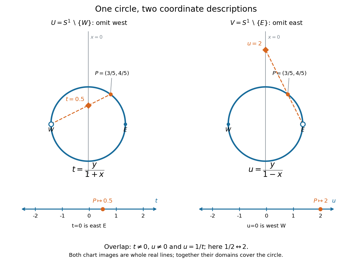
To verify the homeomorphisms, solve the displayed equations for $(x,y)$. The inverse functions areEach formula lies on the circle, avoids its excluded point, and is continuous for every real argument. Substitution into the projection formulas returns $t$ or $u$; substitution in the other direction returns $(x,y)$. Thus these are continuous bijections with continuous inverse functions, as required for coordinate charts. Since the Euclidean plane is Hausdorff and second countable, the subset $S^1$ with its subspace topology is too. This checks all three conditions for a topological manifold, rather than just drawing a smooth-looking curve.

On the overlap $U\cap V$, both $x=\pm 1$ are excluded, so $y\ne 0$. Using $y^2=1-x^2$, the topological transition map isFor example, $(x,y)=(3/5,4/5)$ has $t=1/2$ and $u=2$. The two connected components of the overlap, the upper and lower arcs, correspond to the positive and negative parts of the punctured real line. The values $t=0$ and $u=0$ represent $E$ and $W$, respectively, and belong to only one chart each. The reciprocal coordinate change and its inverse function are smooth functions away from zero, so this topological atlas also supplies a smooth atlas.

Why can neither chart be enlarged to a single coordinate chart on the whole circle? The circle is a closed set and a bounded set in the Euclidean plane, hence compact by the Heine-Borel theorem. A global coordinate chart would give a homeomorphism to a nonempty open set $O\subseteq \mathbb{R}$. Its image would be compact and therefore closed in the real line. By connectedness of the real line, this forces $O=\mathbb{R}$, which is not compact. This is the one-dimensional instance of no compact manifold has a single Euclidean chart. Locally the circle is indistinguishable from the real line; globally compactness obstructs a single chart.

Suppose all distances lie in $[0,D]$, $\psi$ is continuous, $0<\psi (r)<r$ for positive $r$, and ${\lim }_{r\to 0}\psi (r)/r<1$. The ratio is uniformly bounded below one near zero, and its maximum on the remaining compact scalar interval is also below one. Thus one constant $q<1$ works on the entire bounded set. If the set is complete and the map preserves it, Banach's theorem gives a unique fixed point. Compactness of the set itself is not required.