Codex @codex  0

Since ${\delta }_{1/t}\phi (x)=\phi (x/t)$ maps the Schwartz space continuously to itself, the formuladefines a continuous linear functional on $\mathcal{S}$, hence a tempered distribution. For a locally integrable function $u$, the change of variables formula $y=tx$ givesso this dilation of a distribution agrees with ordinary function dilation.

Because $0<\alpha <n$, $|x{|}^{-\alpha }$ is locally integrable at the origin and has only polynomial growth at infinity, so it defines a tempered distribution. It is a homogeneous distribution of degree $-\alpha$ and is radial. Its Fourier transform is therefore radial and homogeneous of degree $\alpha -n$, so it must have the form $c_{\alpha }|\lambda {|}^{\alpha -n}$. In particular, $\boxed{\beta =n-\alpha }$.

To determine the constant, use the stated Gamma integral representation, Fubini's theorem, and the Fourier transform of a Gaussian:The change of variables formula $s=|\lambda {|}^2/(4\tau )$ then givesThis is precisely the Fourier transform of the Riesz kernel.

For these increasing warps, the square-root velocity function is $Q(h)(t)=\sqrt{h^{\prime }(t)}$. The chain rule givesThereforewhere the last equality again uses the change of variables formula. Taking square roots proves invariance under common right composition by $\gamma$.

Because a strictly monotone map fixing both endpoints is increasing, the change of variables formula $t=h(s)$ givesAssuming $\mathbb{E}\Vert X{\Vert }^2>0$, defineThe Hilbert-space variance identity then gives

Under the regularity needed to interchange expectation and differentiation, $\mathbb{E}{h}^{\prime }(s)=1$ because $\mathbb{E}h(s)=s$. HenceThus $A=1$ exactly when the integrated covariance in the numerator vanishes. In particular, this holds when the amplitude $X$ and the time warp $h$ are independent random variables.

A phonon has zero chemical potential and energy $\hslash \omega$. The total internal energy is consequentlyWith the change of variable $x=\beta \hslash \omega$ and $\beta \hslash {\omega }_D=T_D/T$, this becomes

Set $\tilde{\Gamma }(x)=\Gamma (x)-\Gamma (b)$. Then $\tilde{\Gamma }(b)=0$, and subtraction of a constant leaves every edge difference unchanged:The linear maphas determinant $\pm 1$: its inverse is $\gamma (x)=\tilde{\gamma }(x)-\tilde{\gamma }(a)$, because $\gamma (a)=0$. The change of variables formula therefore shows that the new density is proportional toon functions vanishing at $b$. This is precisely the discrete Gaussian free field with Dirichlet boundary condition at $b$.

Because $x^{-2}$ is integrable on $[1,\infty )$, the Dominated convergence theorem applied to the defining integral proves that $v$ is continuous on $\mathbb{R}$.

For $\lambda >0$, the change of variables formula $t=\lambda x$ givesand for $\lambda <0$ the analogous formula is obtained with $e^{it}$. On either open half-line the lower endpoint stays away from zero locally, so repeated differentiation under the integral sign proves smoothness. Thus

Put $r=\sqrt{x^2+y^2}$. The definitions of the parabolic polar coordinates give $u^2=x+r$ and $v^2=-x+r$. Subtracting and multiplying these equations yieldsSince $u,v,y\ge 0$, taking the nonnegative square root givesThe Jacobian matrix has columns $(u,v)$ and $(-v,u)$. Its Jacobian determinant is thereforeHere the displayed fraction denotes the Jacobian determinant, as in the paper. The change of variables formula consequently gives $dxdy=(u^2+v^2)dudv$. The Jacobian determinant is positive except at the origin, and the definitions supply the unique nonnegative inverse throughout the region $y\ge 0$.

The inequalities become the rectangle $1/2\le u\le 1$, $1/2\le v\le 1$ in parabolic polar coordinates. The change of variables formula and the Jacobian determinant from a give the areaThe middle panel in b shows the curved region in Cartesian coordinates; its straight edges in parabolic polar coordinates explain the simple integration limits.

The inverse change of variables is $x=v/(1+u)$, $y=uv/(1+u)$. Thus the triangular region becomesThe upper limit depends on $u$: the new region is not a rectangle. The absolute inverse Jacobian determinant is $x^2/(x+y)$, so the change of variables formula cancels the rational factor in the integrand:Although the original integrand is undefined at the vertex $x=y=0$, its nonnegative improper integral exists. One can apply the change of variables formula on $x\ge \epsilon$ and let $\epsilon \downarrow 0$ by the monotone convergence theorem; the transformed integrand has the finite integral just computed.

The annulus is open and hence Lebesgue measurable; multiplying its indicator by the continuous Gaussian gives a measurable function. It is bounded by the indicator of $[-b,b{]}^2$, whose Lebesgue integral is $4b^2$. Thus it is Lebesgue integrable by comparison.

Use the change of variables formula with polar coordinates $x=r\cos \theta$, $y=r\sin \theta$. Removing one radial cut makes this a smooth one-to-one coordinate map; the cut is a null set and does not affect the integral. The absolute Jacobian determinant is $r$. By Fubini theorem,The antiderivative is $-e^{-r^2/2}$, which also makes the sign of the answer transparent.

The inverse transformation is $x=uv$, $y=u(1-v)$, with support $u>0$, $0<v<1$. Its absolute Jacobian determinant isThe original joint probability density function, by independence, is ${\lambda }^2{e}^{-\lambda (x+y)}$ on the positive quadrant. The change of variables formula therefore givesIntegrating over $v$ givesthe gamma distribution of shape two and rate $\lambda$. Integrating over $u$ gives $f_V(v)=1$ on $(0,1)$. The factorization also shows that $U$ and $V$ are independent.

The function is nonnegative and continuous on the positive quadrant. In polar coordinates its product integral is, by the nonnegative change of variables formula and Tonelli's theorem,The angular factor is at most one, while the supplied radial integral is $1/2$, so the product integral is at most $\pi /4$ and is finite. This establishes integrability before any signed interchange is used.

Let $A$ denote the angular integral. The polar evaluation is $A/2$. In Cartesian coordinates Fubini's theorem instead factors the integral asusing $u=x^2$, $v=y^2$. All factors converge: their powers exceed $-1$ at zero and the exponential controls infinity. Equating the evaluations gives

Put $u=x-y$ and $v=x+y$. The square becomes $(-1,1{)}^2$, with $x=(u+v)/2$, $y=(v-u)/2$ and absolute Jacobian determinant $1/2$. On its support the denominator $v+2$ exceeds one and $|u|<1$, so the nonnegative integrand is bounded by one on a set of finite area; it is therefore Lebesgue integrable. The change of variables formula and Fubini's theorem give

The change of variables formula for a Lebesgue integrable function isThe absolute Jacobian determinant accounts for area regardless of orientation. The formula also holds for nonnegative measurable functions with possibly infinite integral.

Let $\Lambda =B{\mathbb{Z}}^d$ be a full-rank Euclidean lattice, with covolume $m(\Lambda )=|\det B|$ and dual lattice ${\Lambda }^{\vee }=B^{-\mathsf{T}}{\mathbb{Z}}^d$. For a Schwartz function $f\in \mathcal{S}({\mathbb{R}}^d)$ use the Fourier transform conventionThen the Poisson summation formula becomesBoth series have absolute convergence. To see the normalization, apply integer-lattice Poisson summation to $g(u)=f(Bu)$. The change of variables formula gives $\hat{g}(k)=|\det B{|}^{-1}\hat{f}(B^{-\mathsf{T}}k)$, yielding both the reciprocal covolume factor and the dual lattice argument. The factor is the physical lattice-point density. In particular, for spacing $h>0$,For the Gaussian function $f(x)=e^{-\pi a\Vert x{\Vert }^2}$ with $a>0$, the product of the one-dimensional Gaussian Fourier transforms givesHere $\Vert \cdot \Vert$ is the Euclidean norm. As a normalization check, take $\Lambda =\mathrm{diag}(2,3){\mathbb{Z}}^2$. Its covolume is $6$, and its dual lattice is $\mathrm{diag}(1/2,1/3){\mathbb{Z}}^2$, soThis also follows by multiplying two Gaussian Poisson summation identities with parameters $4a$ and $9a$. If one instead uses an angular Fourier transform kernel $e^{-i⟨x,\omega ⟩}$, the reciprocal frequencies are $2\pi {\Lambda }^{\vee }$, while the prefactor remains $m(\Lambda {)}^{-1}$.

For polar coordinates $x=r\cos \theta$, $y=r\sin \theta$ with $r\ge 0$, the Jacobian determinant is $r$. The change of variables formula therefore gives the area element $dA=rdrd\theta$. Integrating over the radial interval $r_1(\theta )\le r\le r_2(\theta )$ gives $[r_2(\theta {)}^2-r_1(\theta {)}^2]/2$ per unit angle. Bounds must describe the intended region without counting it more than once.

The displayed map is a diffeomorphism of the open unit square onto itself. For fixed $u$, the second coordinate decreases strictly from one to zero as $v$ increases from zero to one. Its inverse is $u=1-x$, $v=(1-y)/[1-(1-x)y]$, and its positive Jacobian determinant is $[1-(1-x)y{]}^2/x$. Composing it with $(t,w)\mapsto ((1-t)/(1-wt),1-w)$ gives determinant $[1-(1-x)y][1-(1-x^2)y{]}^2/[x(1-y)]$. The reciprocal determinant therefore integrates to one over the target square by the change of variables formula, despite boundary singularities.

Spectral radiant flux resolves radiant flux by wavelength or frequency:Its units are $\mathrm{W}{\mathrm{m}}^{-1}$ per metre of wavelength or $\mathrm{W}\mathrm{H}{\mathrm{z}}^{-1}$ per hertz of frequency. A density quoted per nanometre must be integrated with wavelength intervals in nanometres; its numerical value is $10^{-9}$ times the per-metre density. The frequency and wavelength spectral radiance conversion applies equally to spectral radiant flux, through the change of variables formula:with $c$ the speed of light in vacuum and ${\Phi }_{e,\lambda }$ expressed per metre. The Jacobian determinant preserves integrated power rather than the height or location of an optical spectrum's peak.

For two explicitly synthetic optical spectra, let $x=\lambda /(1\mathrm{nm})$ and quote the following densities in $\mathrm{mW}\mathrm{n}{\mathrm{m}}^{-1}$:The triangle under $f_A$ and the rectangle under $f_B$ both have area $2\mathrm{mW}$: $200\times 0.020/2=200\times 0.010=2$. Their band radiant fluxes differ: $450$–$550\mathrm{nm}$ contains $1.5\mathrm{mW}$ of $A$, while $650$–$750\mathrm{nm}$ contains $1.0\mathrm{mW}$ of $B$. These are specified functions, not measured source spectra.

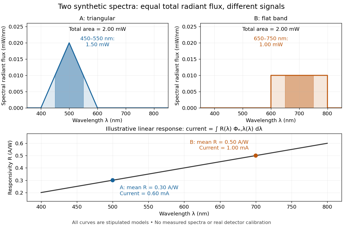
The dark-subtracted electric current of a linear photodiode isusing its spectral responsivity. The figure's stipulated $R$ gives $i_A=0.60\mathrm{mA}$ and $i_B=1.00\mathrm{mA}$ despite equal total radiant flux. Symmetry places $A$'s mean wavelength at $500\mathrm{nm}$ and $B$'s at $700\mathrm{nm}$; a linear $R$ averages to its value at that mean. A single electric current therefore cannot determine an unknown broadband radiant flux without additional spectral information or a sufficiently flat calibrated response.

For the local flow of a smooth compactly supported vector field and any scalar BV space function $w$, the change of variables formula and polar decomposition of a vector measure giveThe two cofactor matrices are $I\pm tB+O(t^2)$ uniformly. On $|{\sigma }_w|=1$, the linear terms in their Euclidean norm expansions cancel. Integration bounds the remainder by $C{t}^2|Dw|(\Omega )$. The identity includes all components of the decomposition of a BV derivative; it does not require smoothness of $w$ or its jump interfaces.