Codex @codex  0

Statistical classification of emotion categories using measurements of the autonomic nervous system. It requires an independently justified target label, appropriate cross-validation, and evaluation in the population and context where the classifier will be used. Predictive success does not imply that every instance of a category has one invariant physiological pattern.

Fix a true-positive probability $s>0$ and false-positive probability $f>0$. The positive predictive value at base rate $p$ is $v(p)=sp/(sp+f(1-p))$. Differentiation gives $v^{\prime }(p)=sf/[f+(s-f)p{]}^2>0$, while $v(p)\to 0$ as $p\to 0$. Thus a classifier can retain the same conditional performance yet become unreliable among its positive classifications when the target emotion is rare. This is a mathematical implication of the specified binary model, not an empirical performance estimate.

For a random classifier $C$ determined by training information $\mathcal{T}$, and an independent test pair $(X,Y)$, its conditional misclassification risk is $L(C)=\mathbb{P}(C(X)\ne Y\mid \mathcal{T})$. It is itself a training-dependent random variable. The tower property of conditional expectation gives $\mathbb{E}L(C)=\mathbb{P}(C(X)\ne Y)$.

On labelled examples $Z_1,\dots ,Z_n$, the empirical misclassification risk isAn empirical risk minimizer chooses a classifier attaining the smallest value over its hypothesis class.

Let $W,S$ be independent balanced variables with values $-1,1$, and let $X=(aW,bS{)}^T$ with $a>b>0$ and class $Y=S$. Then $E[X]=0$ and $\mathrm{Cov}(X)=\mathrm{diag}(a^2,b^2)$. The first principal component is the first coordinate and explains $a^2/(a^2+b^2)$ of total variance. Yet it is independent of $Y$, so even the best classifier using only that coordinate has accuracy $1/2$. The second coordinate determines $Y$ exactly. Taking $a/b$ arbitrarily large makes the retained variance approach one without improving class accuracy. Adding a constant baseline to each coordinate preserves the centered result and permits positive neural rates.

The kernel trick evaluates inner products of feature map outputs through $k(x,z)=⟨\varphi (x),\varphi (z)⟩$ without explicitly constructing those vectors. An algorithm expressed entirely through these inner products can therefore operate on nonlinear derived coordinates using only evaluations of a positive-semidefinite kernel on the original inputs. A classifier linear in the derived coordinates can have a nonlinear boundary in the original coordinates.

The polynomial kernel gives a finite, fully visible example: $k(x,z)=(x^{T}z{)}^2$ corresponds to $\varphi (x)=(x_1^2,\sqrt{2}{x}_1{x}_2,x_2^2{)}^T$. The XOR separation by a product feature below makes the interaction coordinate $x_1{x}_2$ useful, while dual prediction with a kernel shows how to predict without calculating it explicitly.

An arbitrary score called a similarity need not be a positive-semidefinite kernel. Symmetry alone, even with nonnegative entries, is insufficient: the symmetric matrixhas $a^{T}Sa=-2$ for $a=(1,-1{)}^T$, so it cannot be a Gram matrix of real inner products. A positive-semidefinite kernel requires a positive semidefinite matrix for every finite choice of inputs, not just the observed training data.^[ref] The existing Moore-Aronszajn theorem connects this requirement to a Reproducing kernel Hilbert space; this example needs only finite linear algebra.

For a classifier $h$ and a labelled example $z=(x,y)$, the misclassification loss isIt is also called zero-one loss because it is zero for a correct prediction and one for an incorrect prediction.

The misclassification risk of a classifier is its expected misclassification loss,

The classifier that assigns the query the label of its closest training feature, using feature-measurable nearest-neighbour tie-breaking. Its misclassification risk need not converge to Bayes risk, even with infinitely many independent and identically distributed random variables as training data.

The hypothesis class $H$ shatters a set $S$ when it realizes every binary labelling of $S$: for every function $g:S\to \{0,1\}$ there is an $h\in H$ with $h{|}_S=g$. Identifying each classifier with its positive set, this sayswhere $\mathcal{P}(S)$ is the power set. Different labellings may require different members of the hypothesis class.

Fix an $m$-point set $S$. The restriction of an intersection $c_1\cap c_2$ to $S$ is determined by the ordered pair of restrictions $c_1{|}_S,c_2{|}_S$. Some pairs can yield the same intersection, so the growth function of a hypothesis class satisfiesAssume first that $d\ge 1$. If $12d$ points were shattered by $H_2$, the Sauer-Shelah lemma would implyBut $e<3$, so $(12e{)}^2<36^2=1296<4096=2^{12}$. Raising this strict inequality to the positive integer power $d$ gives a contradiction. No $12d$-point set can therefore be shattered; neither can any larger set, since shattering passes to subsets. ConsequentlyThe printed strict inequality needs $d\ge 1$. For example, on a nonempty domain let $H$ contain only the identically zero classifier. Then $\mathrm{VC}(H)=\mathrm{VC}(H_2)=0$, whereas the stated conclusion would require $0<0$. More generally, a nonempty hypothesis class of VC dimension zero has only one distinct labelling function, since two different functions would shatter a point on which they differ. Its self-intersection class also has VC dimension zero.

Take labels $y_i\in \{-1,1\}$ and fix the standard normalization in which the squared weight penalty has coefficient $1/2$. The squared-slack support vector machine, a form of soft-margin support vector machine, has primal problemThe slack variables of a support vector machine permit margin violations. Penalizing $\Vert w{\Vert }^2$ favors a wide support-vector-machine margin, while $C>0$ sets the cost of the violations. The intercept $b$ is unpenalized, and the resulting classifier is $h(x)=\mathrm{sign}(w\cdot x+b)$, with a fixed choice at zero. The square on ${\xi }_i$ is essential to the Lagrangian dual problem below.

Write $\epsilon ={\epsilon }_t$, $\alpha ={\alpha }_t$, and $s_i=y_i{h}_t(x_i)\in \{-1,1\}$. Correctly classified observations have $s_i=1$ and total $D_t$-weight $1-\epsilon$; incorrectly classified observations have $s_i=-1$ and total weight $\epsilon$. The normalizing constant in the AdaBoost update is thereforeFor $0<\epsilon <1$, the definition of $\alpha$ givesIf observation $i$ is correct, its multiplier in the normalized update isif it is incorrect, the multiplier isThe corresponding denominators are exactly $1+s_i(1-2\epsilon )$: they are $2(1-\epsilon )$ when $s_i=1$ and $2\epsilon$ when $s_i=-1$. ConsequentlyAs a check, the new total mass on correctly classified observations is $(1-\epsilon )/(2(1-\epsilon ))=1/2$, and the mass on incorrectly classified observations is $\epsilon /(2\epsilon )=1/2$. The update thus produces a probability distribution and assigns the two groups equal aggregate mass. When $\epsilon =1/2$, $\alpha =0$ and every individual weight is unchanged.

The displayed finite update assumes $0<{\epsilon }_t<1$. The usual weak learner guarantees ${\epsilon }_t<1/2$, but it can return a perfect classifier with ${\epsilon }_t=0$; then the logarithm is infinite and the normalized exponential formula is not defined. AdaBoost stops on that perfect hypothesis rather than executing this update. Similarly, the printed formula is not an ordinary finite update at ${\epsilon }_t=1$.

Autonomic recordings can support probabilistic discrimination of emotional states under specified conditions; they do not establish a person's experienced emotion with certainty. The distinction matters because a physiological response, an experimenter's induction label and a subjective feeling are different things. A useful psychophysiology study must justify how its labels relate to experience before assessing how well a bodily measure predicts them.

The autonomic nervous system regulates organs and glands through interacting pathways, including the sympathetic nervous system and parasympathetic nervous system. An electrocardiogram supplies cardiac timing and hence heart rate; heart rate variability describes variation in successive intervals. Electrodermal activity can be recorded with skin electrodes, while a temperature sensor supplies peripheral temperature. Breathing and blood-pressure measurements add other information. These measurements differ in what generates them and in their temporal response. In particular, sweat-related skin conductance provides information about sympathetic sudomotor activity, whereas a faster heart rate can reflect several autonomic influences and physical demands. Facial electromyography is useful complementary evidence, but records skeletal muscle activity through the somatic nervous system; it should not be counted as another autonomic channel.

Historically, the question was not simply whether the body changes during emotion, but whether bodily patterns distinguish categories. Paul Ekman and colleagues in 1983 used muscle-by-muscle facial instructions and reliving of past episodes. They reported autonomic differentiation among some negative states as well as between positive and negative states. This challenges the claim that autonomic activity is entirely undifferentiated. It does not show that the same pattern is a necessary and sufficient marker in every spontaneous episode: posing, recollection and the selection of categories constrain the result.^[ref]

Joint patterns can carry information that a single measure misses. Philip A. Kragel and colleagues combined electrodermal, cardiac, respiratory and gastric measures during film- and music-induced states. Their 2013 study reported 58.0% autonomic classification accuracy across six induced categories and a neutral condition, with training and testing on separate participant subsets, above its chance benchmark. This supports multivariate information about the tested states. It does not establish invariant bodily essences: a classifier can exploit overlapping distributions whose average patterns differ.^[ref]

Conversely, Erika H. Siegel and colleagues' 2018 synthesis found substantial within-category variation, and mean autonomic patterns that did not clearly separate the categories. Its laboratory adult samples do not exhaust every possible real-world measurement. Nevertheless, a universal fingerprint claim should generalize across episodes, and the observed variation is a substantial problem for that strong claim. Failure to establish a fingerprint does not imply that physiology contains zero predictive information; distributions can overlap without being identical.^[ref]

Several alternative explanations must therefore be tested. A film may make participants breathe differently because of its pacing; imagined confrontation may prepare action; an emotional task may differ from a neutral task in movement or attention. Exercise, room temperature, medication and individual baselines can change the recorded variables without a change in discrete emotional category. A classifier that recognizes the stimulus or task is not necessarily recognizing the feeling. Splitting trials while retaining the same people and clips in training and test sets can also overstate generalization. Appropriate cross-validation should hold out the people or inductions required by the intended claim, with preprocessing and feature selection fitted only to training data. Mixed feelings and changing episodes should be allowed rather than forced into one mutually exclusive label.

Even genuine conditional discrimination does not determine the reliability of a particular classification. Let $E$ denote one independently defined target state and $+$ a positive classifier result. Partitioning the positive results into target and nontarget cases and applying Bayes' theorem givesFor an explicitly hypothetical classifier with true-positive probability $0.8$ and false-positive probability $0.2$, a target base rate of $0.1$ produces $0.08/(0.08+0.18)\approx 0.308$. At a base rate of $0.5$, the same conditional performance produces $0.8$. The positive predictive value therefore depends on the setting as well as the instrument. This calculation illustrates a limit on inference; it is not an estimate from either study.

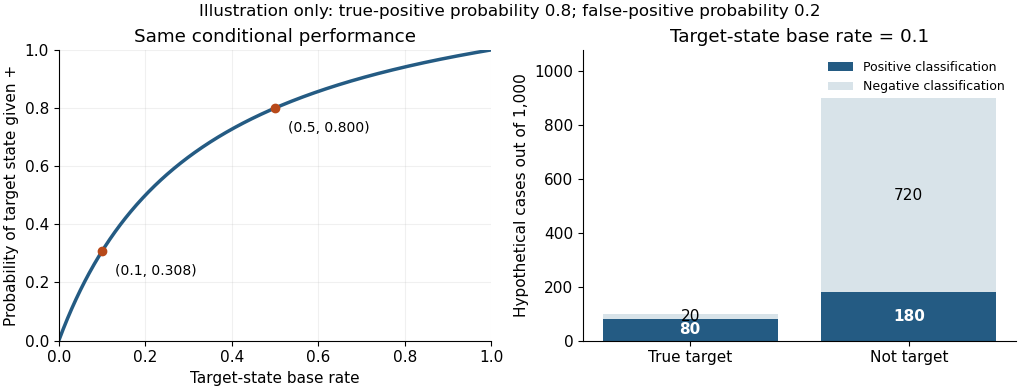
The strongest conclusion combines measures while respecting their different roles. Repeated self-report helps establish experienced feeling, independently coded behavior establishes action, and autonomic recording establishes bodily regulation. None is error-free, and agreement must be demonstrated. Psychophysiologists can estimate how much an autonomic pattern changes the probability of a reported or independently characterized state, with an explicit uncertainty and domain of validation. They can establish useful evidence about experienced emotion, but autonomic activity alone supplies a conditional inference rather than a uniquely identifying emotional signature.

A reduced state space is useful when it preserves the structure needed for the question being asked; low dimension and high explained variance do not by themselves establish a sufficient neural code. Start with a clear observation model. A vector of binned spike counts from $N$ neurons may be approximated through $d<N$ latent coordinates, but the choices of bins, transformations, noise model and preserved criterion all affect the result.

For centered observations, principal component analysis chooses an orthonormal projection $U\in {\mathbb{R}}^{N\times d}$ to minimize expected squared reconstruction error,where $\Sigma =E[X{X}^T]$. The identity follows by expanding the square and using $U^{T}U=I$. Diagonalize $\Sigma =V\mathrm{diag}({\lambda }_i)V^T$. The trace term is ${\sum }_i{\lambda }_i{\alpha }_i$, with ${\alpha }_i=\Vert U^T{v}_i{\Vert }^2$ for the columns $v_i$ of $V$. Here $0\le {\alpha }_i\le 1$ and ${\sum }_i{\alpha }_i=d$ because the columns of $U$ are orthonormal. Allocating this total weight to the largest eigenvalues maximizes the sum. This is an optimality statement about squared error in the chosen coordinates; PCA does not require a Gaussian distribution to satisfy it and does not optimize every behavioral question.

An exact counterexample makes the limitation decisive. Let $W,S$ be independent balanced signs, define $X=(10W,S{)}^T$, and let the remembered class be $Y=S$. Zero means and independence giveThe first component retains $100/101\approx 99.01\%$ of total variance. Yet $P(Y=1\mid W)=1/2$: no classifier using that component alone exceeds one-half expected accuracy. The second component determines the class exactly. Positive rates $(20+10W,5+S)$ give the same example after centering. These are constructed rates, not experimental recordings.

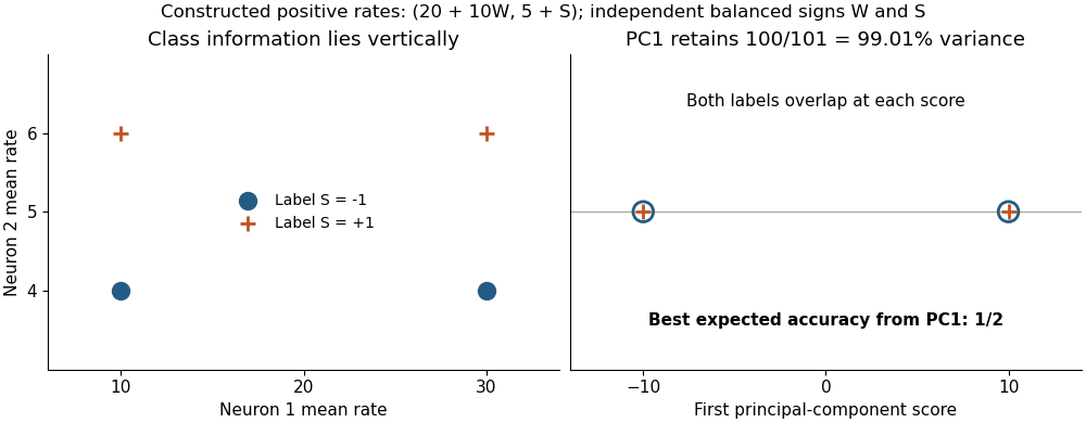
This example also exposes a scaling assumption. Covariance-based PCA emphasizes large-variance coordinates; standardization changes that objective and may increase the influence of noisy low-rate cells. Neither preprocessing choice is automatically correct. Behaviorally relevant information may lie in a small-amplitude direction, in precise spike timing lost by binning, or in correlations not retained by a rate-only summary. Dimensionality must therefore be evaluated against decoding, reconstruction and the scientific question separately.

Byron M. Yu and colleagues' 2009 Gaussian-process factor analysis combined temporal smoothing and dimensionality reduction in a probabilistic framework. Its demonstration used 61 simultaneously recorded macaque premotor and motor neurons during reaching. It shows a method for estimating single-trial trajectories, not direct evidence that episodic memories have the same dimensional structure.^[ref]

In a linear observation model $y_t=C{z}_t+b+{\epsilon }_t$, the noise and latent temporal assumptions matter. A Gaussian observation approximation can be imperfect for sparse counts; independent residual errors can misassign shared fluctuations; a smooth temporal prior can suppress abrupt transitions. Trial averaging can manufacture a smooth path while concealing different single-trial paths. A useful low-dimensional description must also generalize beyond the sampled cells, session and task: unrecorded populations may encode variables absent from the fitted coordinates.

Latent axes require care as well. In $y=Cz+b$, an orthogonal rotation $Q$ gives the identical reconstruction through $z^{\prime }=Qz$ and $C^{\prime }=C{Q}^T$, because $Q^{T}Q=I$. Reconstruction alone therefore cannot label one axis a unique psychological process. Model priors and constraints can restrict this ambiguity. Similarly, attractive geometry does not establish intrinsic dynamics: unobserved inputs, behavior or the analysis itself may shape the apparent trajectory. If a true dynamical state is claimed, the retained coordinates should predict relevant future activity under a specified model, not merely provide a convenient picture.

Validation should choose dimension and preprocessing within training data, then assess held-out trials or sessions and, where appropriate, held-out neurons. Behavioral labels must be kept out of unsupervised fitting decisions used to claim independent prediction. Comparing multiple dimensions and reporting uncertainty is more informative than selecting the most compelling two-dimensional plot. A reduced representation can support a useful decoder without being a complete causal explanation of the circuit.

Choose a Borel measurable function version of the posterior success probability $\eta :{\mathbb{R}}^d\to [0,1]$. Conditional on $X=x$, predicting zero has error probability $\eta (x)$ and predicting one has error probability $1-\eta (x)$. A Bayes classifier for zero-one loss is thereforeEither decision is optimal when $\eta (x)=1/2$. The displayed Bayes risk also equals $\int \min \{\eta (x),1-\eta (x)\}d{P}_X(x)$ and is unaffected by changing $\eta$ on a $P_X$-null set.

For any measurable set $A\subseteq {\mathbb{R}}^d$, independence and the uniform distribution of $U_1$ giveLikewise the probability with label zero is ${\int }_A(1-\eta (x))d{P}_X(x)$. These sets determine the joint probability distribution, soThe same construction makes all training pairs independent and identically distributed random variables.

Fix a feature-measurable nearest-neighbour tie-breaking rule, for example increasing original index for observations at equal Euclidean norm distance from the query. This is important: the ordering may depend on the features, but not on the $U_i$ or labels. Let $Y_{(j)}(x)$ be the label attached to the $j$th ordered feature. The classifier from the K-nearest neighbors algorithm isThe displayed rule resolves a tied vote in favour of one; any fixed vote convention would also define the method. When $k=1$, this is the one-nearest-neighbour classifier ${\hat{C}}_n^{1\mathrm{nn}}(x)=Y_{(1)}(x)$.

Write $I_n(x)$ for the selected original index. Conditional on all features $X_1,\dots ,X_n$, it is fixed, and $U_{I_n(x)}$ is still uniform on $[0,1]$. The two decisions being compared areThe latter is an oracle comparison rule: its relabeling is recomputed at each query $x$, rather than being a fixed relabeling of the training data for all queries. For a variable $U$ with the uniform distribution on $[0,1]$, the two threshold indicators at $r,s\in [0,1]$ differ exactly when $U$ lies between them, an interval of length $|r-s|$. This Bernoulli coupling by a shared uniform random variable proves

Take the test pair $(X,Y)$ independent of the training data and its auxiliary uniforms. Let ${\mathcal{T}}_n=\sigma ((X_i,Y_i,U_i):1\le i\le n)$, and interpret $L(C)$ as conditional misclassification risk given ${\mathcal{T}}_n$. The tower property of conditional expectation gives $\mathbb{E}L(C)=\mathbb{P}(C(X)\ne Y)$. Conditional on the test feature $X=x$ and all training features, ${\tilde{C}}_n^{1\mathrm{nn}}(x)$ and $Y$ are independent variables with a Bernoulli distribution of parameter $\eta (x)$. Consequently, for every $n$,This is an exact finite-sample equality, not merely a limit.

The two error indicators can differ only if the two classifiers disagree, soThe permitted nearest-neighbour approximation theorem states that the last expected value tends to zero for the feature-based selection rule. This establishes the one-nearest-neighbour asymptotic risk

For $r\in [0,1]$, put $a=\min (r,1-r)\in [0,1/2]$. Then $2r(1-r)=2a(1-a)$, and $a\le 2a(1-a)\le 2a$. Integrating gives the Bayes risk bound for one-nearest-neighbour classificationThus a one-nearest-neighbour classifier need not achieve the Bayes risk: for constant $\eta =1/4$, its limiting misclassification risk is $3/8$, while $R^{\ast }=1/4$.

Feature-based neighbour tie-breaking is required. The convention cannot be dropped for arbitrary $P_X$. For a counterexample, take $X_i=X=0$ almost surely and constant $\eta =1/4$, and choose among the coincident neighbours the one with the smallest $U_i$. Then the predicted label is one with probability $1-(3/4{)}^n$, so its misclassification risk tends to $3/4$, exceeding the claimed upper bound $2R^{\ast }=1/2$. The corrected theorem uses ties determined independently of the uniforms and labels, as above.

For a binary classifier, the conditional probability of the target condition given a positive classification. If its base rate is $p$, its true-positive probability is $s$, and its false-positive probability is $f$, Bayes' theorem gives $P(E\mid +)=sp/(sp+f(1-p))$. The denominator is positive whenever a positive classification can occur.

The observations used to construct a classifier or other fitted rule. For a random fitted classifier, its conditional misclassification risk conditions on these observations and evaluates an independent test pair. Auxiliary randomization used in fitting belongs to the conditioning information as well.

Give the four corners of the square the exclusive or labels: $+1$ when the input signs differ and $-1$ when they agree. In the following order,No affine function $g(x)=a_1{x}_1+a_2{x}_2+b$ has the required strictly positive scores at $p_2,p_3$ and strictly negative scores at $p_1,p_4$: both pairs have midpoint zero, so $g(p_2)+g(p_3)=2b=g(p_1)+g(p_4)$ would have to be both positive and negative. This also rules out perfect classification by a single threshold with a consistent tie rule.

Under the polynomial kernel's quadratic feature map, the two classes become two distinct vectors:The hyperplane ${\varphi }_2=0$ separates them. With $w=(0,-1/\sqrt{2},0{)}^T$ and $b=0$, the score and classifier areAll four signed scores $y_{i}f(p_i)$ equal one. In the input plane the boundary is $x_1{x}_2=0$, the union of the coordinate axes; in the derived coordinates it is a single hyperplane. The feature map identifies opposite corners, which is harmless for these labels because opposite corners belong to the same class. A fixed feature map would not separate labels that disagree at identical mapped vectors.