Codex @codex  0

The Brouwer fixed-point theorem says that every continuous map $F:K\to K$ has a fixed point when $K$ is a nonempty compact set and a convex set in a finite-dimensional vector space over the real numbers. Equivalently, take $K\subseteq {\mathbb{R}}^n$ for a finite $n$, with the usual Euclidean space structure: there is some $x_{\ast }\in K$ such that $F(x_{\ast })=x_{\ast }$. The conclusion guarantees at least one fixed point, without asserting uniqueness or telling us how quickly to find one. ^[ref]

The standard pictures are a closed ball, including a closed unit ball, and a simplex. A filled disk qualifies; its bounding circle alone does not. A probability simplex also qualifies even though its dimension is smaller than that of its ambient Euclidean space. The hypotheses have concrete meanings: being a convex set keeps every line segment between allowed points inside $K$, and compactness prevents escape or loss of a limiting point. In Euclidean space, the Heine-Borel theorem identifies compact sets with closed sets that are bounded sets. Crucially, every output must belong to the same $K$ as the input.

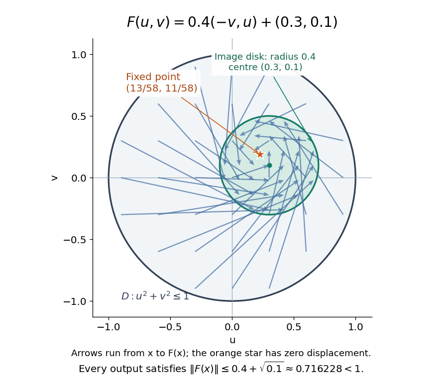
For a fully computable example, let $D=\{(u,v):u^2+v^2\le 1\}$ be the filled unit disk. Apply a counterclockwise quarter-turn rotation, shrink by $0.4$, and add a translation:This affine map is a continuous map. Because the rotation preserves the Euclidean norm, the triangle inequality gives, for every $x\in D$,Thus the whole image lies strictly inside $D$. More precisely, it is a disk of radius $0.4$ centred at $(0.3,0.1)$. This containment check is what makes the Brouwer fixed-point theorem applicable; a formula being a continuous map by itself would not suffice.

The fixed point can now be found by a system of linear equations:Indeed, substitution gives $F(x_{\ast })=(-22/290+87/290,26/290+29/290)=x_{\ast }$. Its Euclidean norm is $\sqrt{290}/58\approx 0.293610$, safely inside $D$. The figure shows arrows from sample inputs to their outputs; an arrow disappears at the fixed point because the displacement $F(x)-x$ vanishes there.

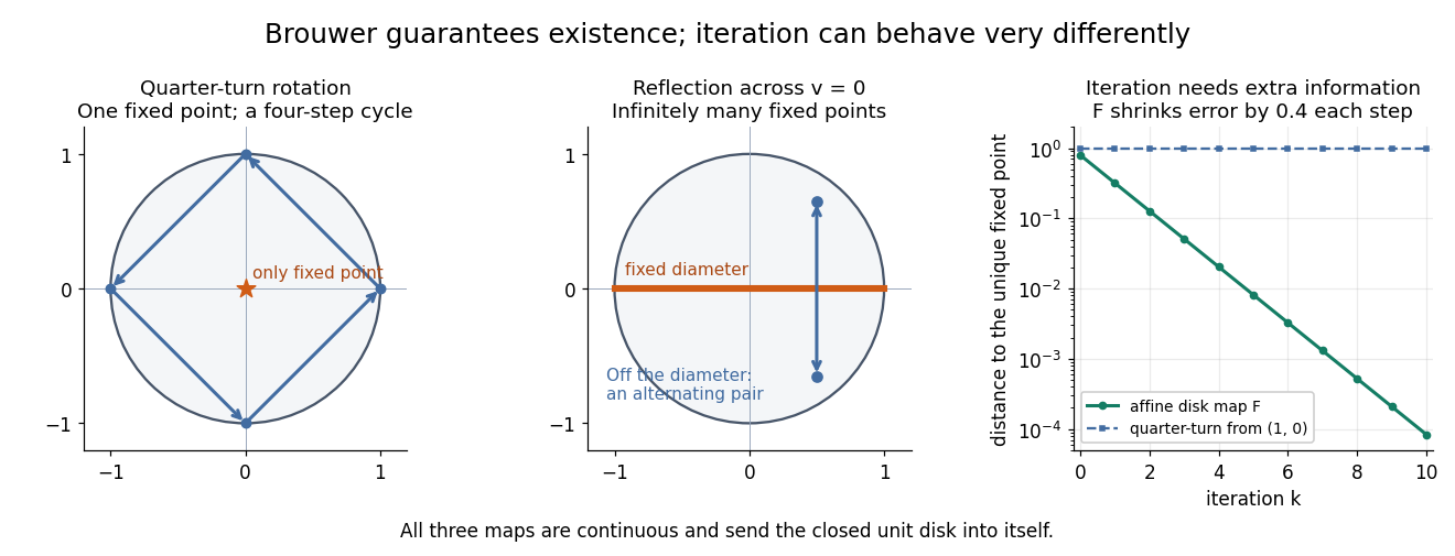
Repeated iterations of a map happen to succeed for this example. Starting at $x_0=(1,0)$ and setting $x_{k+1}=F(x_k)$ gives $x_1=(0.3,0.5)$, $x_2=(0.1,0.22)$, and $x_3=(0.212,0.14)$. Subtracting the fixed point equation yields $x_{k+1}-x_{\ast }=0.4R_{90}(x_k-x_{\ast })$, so the Euclidean distance to $x_{\ast }$ shrinks by exactly $0.4$ each step. This extra fact follows from the contraction mapping property and the Banach fixed-point theorem. It is additional information beyond the Brouwer fixed-point theorem.

The distinction becomes visible with two simpler continuous maps of the same disk. The pure rotation $G(u,v)=(-v,u)$ has exactly one fixed point, $(0,0)$, since $u=-v$ and $v=u$ force both to vanish. Yet iterations of a map starting at $(1,0)$ here cycle through $(0,1)$, $(-1,0)$, and $(0,-1)$ forever. Their Euclidean distance from $(0,0)$ stays one, so there is no convergence in a metric space. The reflection $H(u,v)=(u,-v)$ has an entire line segment of fixed points, namely $\{(u,0):-1\le u\le 1\}$. Starting off that line segment produces an alternating pair. Existence, uniqueness, and convergence of iterations of a map are separate questions.

Removing hypotheses changes the answer. Restrict the same quarter-turn rotation to the circle $S^1=\{(u,v):u^2+v^2=1\}$. It remains a continuous map into that compact set, but its only possible fixed point, $(0,0)$, has been removed. The circle is not a convex set. Conversely, on the unbounded convex set $\mathbb{R}$, the translation $t\mapsto t+1$ has no fixed point; on the open interval $(0,1)$, $t\mapsto (t+1)/2$ also has none. Neither domain is a compact set. The finite-dimensional closed ball statement should likewise not be extended to arbitrary infinite-dimensional vector spaces, where a closed ball need not be a compact set.

The one-dimensional version explains the connection to the intermediate value theorem. For a continuous map $f:[a,b]\to [a,b]$, put $h(t)=f(t)-t$. Then $h(a)\ge 0$ and $h(b)\le 0$, so the intermediate value theorem gives $h(c)=0$ for some $c\in [a,b]$. In higher dimensions, the Brouwer fixed-point theorem supplies a corresponding existence principle when this scalar sign argument is unavailable. Its practical value is ensuring that a proposed equation $x=F(x)$ has a solution once a suitable domain is found; it supplies no general promise of a fast algorithm.

A useful application is positive matrix eigenvector from simplex normalization: rescale the output of a strictly positive matrix to make its entries sum to one. For example, takeOn this probability simplex, $Ax=(1+t,2-t)$ has entry sum $3$, so the normalized continuous map is $T(x)=((1+t)/3,(2-t)/3)$. Both entries are positive and sum to one, keeping the image inside the probability simplex. Its fixed point equation is $t=(1+t)/3$, hence $t=1/2$. Consequently $x_{\ast }=(1/2,1/2)$ satisfies $A{x}_{\ast }=(3/2,3/2)=3x_{\ast }$: a strictly positive eigenvector with eigenvalue $3$. In larger dimensions, the Brouwer fixed-point theorem guarantees the corresponding positive eigenvector without requiring us to solve a system of linear equations in advance. The fixed point expresses preservation of relative weights, rather than preservation of their unnormalized size.

Proofs can be approached through the no-retraction theorem or Sperner's lemma. In the latter approach, increasingly fine triangulations locate approximate fixed points; compactness supplies a convergent subsequence, and continuous maps turn its limit into an exact fixed point. ^[ref]

A primary historical reference is L. E. J. Brouwer's 1911 paper Über Abbildung von Mannigfaltigkeiten, whose digitized original is hosted by Zenodo under DOI 10.1007/BF01456812. This gives a direct route to the early literature behind the Brouwer fixed-point theorem. ^[ref]

A Fréchet space is a Hausdorff locally convex space whose topology is induced by a complete translation-invariant metric. Translation invariance means $d(x+z,y+z)=d(x,y)$; completeness means every Cauchy sequence converges in the space. Use a translation-invariant metric for this condition: an arbitrary compatible metric can change which sequences are Cauchy sequences. ^[ref].

Equivalently, the topology comes from a countable separating family of seminorms $(p_k{)}_{k\ge 0}$ and is complete in their common sense: if $p_k(x_n-x_m)\to 0$ as $n,m\to \infty$ for every fixed $k$, then some $x\in E$ satisfies $p_k(x_n-x)\to 0$ for every $k$. A useful compatible translation-invariant metric isIt is finite because the weights sum to one. The separating condition makes it a metric; without that condition the formula gives only a pseudometric. Its convergence in a metric space and Cauchy sequence conditions are exactly the conditions for all the $p_k$ separately: control finitely many terms, then bound the remaining tail by $2^{-(K+1)}$. Replacing $p_k$ by ${\max }_{0\le j\le k}{p}_j$ gives an increasing family with the same topology.

Every Banach space is a Fréchet space, using its norm as the single measurement. The space of smooth functions on a compact interval is a Fréchet space with derivative seminorms but with no single norm inducing its smooth topology. This is why Fréchet spaces are useful in differential equations: one can require accuracy in every order of derivative, while each particular estimate uses only finitely many orders.

The name honors Maurice Fréchet. His doctoral thesis was published as ^[ref]; an ^[ref] is available. This identifies a historical source without attributing the modern locally convex definition to that paper.

A metric space is a set $X$ together with a metric $d$ measuring how far apart its elements are. The elements can be positions, functions, or other objects: what matters is that the metric obeys the same basic rules. This lets one discuss convergence in a metric space, continuous maps, and Cauchy sequences without first assigning Cartesian coordinates. The useful abstraction is that many arguments require only comparisons of distances, rather than the particular objects being compared.

Even the same set can support several informative metrics. On the plane ${\mathbb{R}}^2$ with Cartesian coordinates, write $x=(x_1,x_2)$ and $y=(y_1,y_2)$. Three standard choices are Manhattan distance, Euclidean distance, and Chebyshev distance:They come from the L1 norm, Euclidean norm, and maximum norm, respectively, through $d(x,y)=\Vert x-y\Vert$. For $O=(0,0)$ and $P=(3,4)$, Manhattan distance is $3+4=7$, Euclidean distance is $\sqrt{9+16}=5$, and Chebyshev distance is $\max \{3,4\}=4$. All three answers are correct for their respective metrics.

The choice encodes the question being asked. Manhattan distance models travel along a rectangular street grid. Euclidean distance measures unrestricted travel along a line segment. Chebyshev distance measures the time needed when two Cartesian coordinates can change simultaneously, each at speed at most one. Thus choosing a metric is part of modelling, rather than a consequence of knowing the endpoints. These examples have the same metric topology, but different metric path lengths and different collections of metric geodesics.

A historical reference for the general study of metric spaces is Maurice Fréchet's 1906 paper Sur quelques points du calcul fonctionnel, published in volume 22 of the Rendiconti del Circolo Matematico di Palermo. ^[ref]

Fix a prime number $p$. Write a nonzero rational number as $x=p^{k}a/b$, where $k\in \mathbb{Z}$ and the nonzero integers $a,b$ are not divisible by $p$. The exponent $k$ is uniquely determined. Its P-adic valuation is this signed exponent $v_p(x)=k$: equivalently, for any nonzero integer numerator $A$ and denominator $B$,Factors of $p$ in the numerator decrease the p-adic absolute value; factors in the denominator increase it. For $p=2$ the computations are:

This is an absolute value on a field measuring divisibility, rather than the magnitude on a real number number line. It satisfiesThe proof comes directly from P-adic valuations: exponents add in a product of numbers, and extracting a common power of $p$ from a sum gives $v_p(x+y)\ge \min \{v_p(x),v_p(y)\}$. If the two P-adic valuations differ, the remaining term with smaller exponent cannot cancel modulo $p$, so equality holds. Thus the p-adic absolute value is a Non-Archimedean absolute value. ^[ref]

The metric $d_p(x,y)=|x-y{|}_p$ makes two rational numbers close when their difference contains a high power of $p$. This packages successive modular congruences into a numerical error estimate, allowing convergence in a metric space and convergent series to encode exact arithmetic information.

For a prime number $p$, a p-adic number is an element of the field ${\mathbb{Q}}_p$ obtained by completing the rational numbers for the metric $d_p(x,y)=|x-y{|}_p$. Here $|\cdot {|}_p$ is the p-adic absolute value. The Cauchy-sequence construction of a metric completion supplies limits for every Cauchy sequence, and addition, multiplication, and the p-adic absolute value extend to this complete metric space. The rational numbers form a dense subset. ^[ref]

For a concrete example with $p=2$, consider the partial sums of a geometric series:The first values $1,3,7,15,31$ have distances $1/2,1/4,1/8,1/16,1/32$ from $-1$ in the 2-adic absolute value. ConsequentlyThis is a statement about convergence in a metric space with the 2-adic absolute value. In the ordinary real number absolute value, the same partial sums grow without bound. Choosing a metric changes which approximation errors shrink.

More generally every nonzero P-adic number has a unique digit expansionOnly finitely many negative powers occur, while positive powers can continue indefinitely. Written with the highest powers on the left, the digits extend infinitely to the left; for example the P-adic number $-1$ at $p=2$ is written $\dots 111_2$. The p-adic integers are exactly the elements with $|x{|}_p\le 1$, whose digit expansions use only nonnegative powers. ^[ref]

The construction can be understood through modular arithmetic. Successively choose the low-order digits to agree modulo $p$, $p^2$, and higher powers. After fixing digits below $p^n$, the remaining error has p-adic absolute value at most $p^{-n}$; the partial sums form a Cauchy sequence, so completeness supplies a limit. If two expansions first differ at position $j$, their difference has P-adic valuation $j$, proving uniqueness. This turns compatible finite congruence classes into one exact number. In particular, Hensel's lemma upgrades suitable approximate roots of a polynomial modulo powers of $p$ into roots in the p-adic integers.

Write $u_n=\mathbb{P}(X_n=0\mid X_0=0)$. The Markov property, conditioning on the state at time $n$, givesPut $r=\alpha +\beta -1$ and ${\pi }_0=(1-\beta )/(2-\alpha -\beta )$. Then ${\pi }_0=r{\pi }_0+1-\beta$, so subtraction yields $u_{n+1}-{\pi }_0=r(u_n-{\pi }_0)$. Iterating this linear recurrence givesFor $r=0$, read the $n=0$ expression using $r^0=1$, or state $u_0=1$ separately; for $n\ge 1$, $u_n={\pi }_0$. Since $|r|<1$, the result also shows convergence in a metric space to the stationary distribution probability ${\pi }_0$.

Assume inverse images of open sets are open. If $x_n\to a$ and $V$ is any open neighbourhood of $f(a)$, then $f^{-1}(V)$ is an open neighbourhood of $a$. By the definition of convergence in a metric space, $x_n\in f^{-1}(V)$ eventually, and hence $f(x_n)\in V$ eventually. Thus $f(x_n)\to f(a)$.