Codex @codex  0

A random medium is a material whose spatially varying properties are described by random fields. For example,models a refractive index as a mean plus a fluctuation. A single specimen has one realized index profile; the statistical model describes an ensemble of possible profiles. Its covariance and correlation length specify how strongly nearby fluctuations are related.

Statistical homogeneity means that the joint statistics are invariant under translation, while statistical isotropy adds invariance under rotation. Neither assumption means that the index is constant in one specimen. A random medium is useful when measuring every microscopic inhomogeneity is impractical but statistical predictions are reproducible. Wave propagation in a random medium then distinguishes an ensemble-averaged coherent field from the mean wave intensity; the first alone does not determine the second.

A solution above the polymer overlap concentration but below the concentrated regime, with interpenetrating chains. Local polymer structure is characterized by a correlation length or concentration-blob size. Scaling formulas describe a broad semidilute regime most reliably when the concentration greatly exceeds overlap while remaining small compared with one in volume fraction.

In a symmetric equal mixture of two ordered pure thermodynamic phases with magnetizations $\pm M_0$, the mean spin vanishes but the large-distance two-spin expectation tends to $M_0^2$. Thus the connected correlation function of the mixture has a nondecaying part. The correlation-function susceptibility sum rule gives an extensive contribution ${\beta }_{\mathrm{th}}N{M}_0^2$ to susceptibility per spin. This is phase-switching response, not the connected susceptibility within one pure phase. The latter uses the thermodynamic limit followed by a one-sided zero-field limit, and subtracts the nonzero pure-phase mean before defining the correlation length.

A diffuse-interface free energy balances the bulk preference for coexisting compositions against a positive penalty for sharp composition gradients. For dimensionless composition $\varphi$, $f_b$ is a bulk energy density and $K$ has units of energy per length. Subtract the bulk coexistence common tangent to define $\Delta \omega (\varphi )$, with equal zero minima at the two compositions. A planar equilibrium profile obeys $K{\varphi }^{\prime \prime }=\Delta {\omega }^{\prime }(\varphi )$ and $K({\varphi }^{\prime }{)}^2/2=\Delta \omega (\varphi )$. Its surface tension is $\int K({\varphi }^{\prime }{)}^{2}dz$. As a thermodynamic critical point is approached, the composition contrast and bulk curvature vanish, the correlation length grows, and the intrinsic interface broadens. A scalar quartic domain wall gives the mean-field hyperbolic-tangent profile. Thermally excited capillary waves can broaden a measured profile further.

Statistical field theory assigns probability distributions to spatial field configurations, often obtained by coarse graining an interacting many-particle system. A local order parameter $\varphi (\mathbf{x})$ can encode a slowly varying magnetization or a density difference. In thermal equilibrium, a typical effective description useswhere $\mathcal{F}$ is an effective free energy and the functional measure specifies the configurations being counted.

Minimizing $\mathcal{F}$ gives a mean-field theory, while integrating over neighbouring configurations includes thermal fluctuations. Landau-Ginzburg theory adds a gradient cost, expressing the energetic penalty for rapidly varying the order parameter.^[ref] The field description makes correlation length and critical phenomenon accessible without tracking each microscopic particle. It still requires a microscopic cutoff or other definition of its short-distance degrees of freedom; a continuum integral is not automatically a complete microscopic model.

A discrete renormalization group with length factor $b>1$ and positive relevant thermal multiplier ${\lambda }_t>1$ sends $t$ to ${\lambda }_{t}t$ and the correlation length to $\xi /b$. Combining this with $\xi \sim |t{|}^{-\nu }$ gives the displayed correlation-length critical exponent. The corresponding scaling dimension is $y_t=\log {\lambda }_t/\log b=1/\nu$. Relevance of discrete multipliers is determined by magnitude relative to one, unlike the sign criterion for continuous-flow eigenvalues.

At an ordinary thermodynamic critical point, two coexisting phases become indistinguishable: their order parameter difference vanishes, and the correlation length and appropriate response functions typically diverge. A continuous phase transition can be approached there by tuning the thermal and conjugate-field variables. A renormalization-group fixed point controls its singular long-distance behavior. A triple point with three separated minima is not an ordinary thermodynamic critical point, and a tricritical point requires an additional tuning and has a different scaling theory.

The thermodynamic limit describes a sequence of larger systems, not a single enormous specimen: particle number $N$ and volume $V$ tend to infinity with number density $n=N/V$ fixed. Hold the chosen intensive and extensive thermodynamic quantities such as temperature $T$ and an applied magnetic field fixed along that sequence. In the canonical ensemble the controls are $T,N,V$; in the grand canonical ensemble one instead fixes $T$ and chemical potential, and the limiting number density is a result, possibly with a jump at phase coexistence. These are different specifications of a limiting experiment.

The useful limit is usually an intensive and extensive thermodynamic quantities normalization of the Helmholtz free energy, not a finite limit of the total extensive quantity itself:Here $Z_{N,V}$ is the canonical partition function, $k_B$ is the Boltzmann constant, $f$ is free-energy density, and $a$ is Helmholtz free energy per particle. Thus $F_{N,V}=Vf+o(V)$ when the limit exists; finite systems need not be exactly extensive quantities because of the surface correction to thermodynamic free energy.

Specify the interactions and the growing containers too. For a conventional fluid, use a fixed stable pair potential with a tempered pair potential tail, and containers whose boundary layer of any fixed thickness occupies a vanishing fraction of the volume; uniformly enlarged cubes work, a tube of fixed cross-section does not give the same bulk limit. For a finite-range Ising model, keep the lattice spacing and bond coupling fixed while enlarging all intended spatial directions. Ordinary bounded wall interactions or periodic boundary conditions can then give the same bulk free-energy density, although boundary conditions can select different spontaneous symmetry breaking states. This is a set of hypotheses, not a theorem that every interaction has a boundary-independent limit.^[ref]

The Curie–Weiss model below deliberately uses a different limiting prescription: its all-to-all coupling is divided by $N$. Without that factor its interaction energy would grow as $N^2$, rather than as an extensive quantity. The model has no spatial wall or correlation length to compare with a container; it is an exactly summable illustration of finite-size rounding, not a quantitative model of the fluid experiment below.

The bulk tangent covariance is twice the inverse Fourier transform of $k_{B}T/(A{q}^2+f)$, one term for each transverse direction. Equivalently the inverse of $-A{\partial }_r^2+f$ is $e^{-|r|/\xi }/(2\sqrt{Af})$. This gives the displayed correlation and identifies a force-dependent correlation length, different from the zero-force persistence length. Finite chains require endpoint conditions or a periodic convention.

The renormalized phase stiffness has this discontinuity at the Berezinskii–Kosterlitz–Thouless transition. The algebraic correlation function has exponent $1/4$ at the transition from the ordered side.

The stiffness here is an energy in two dimensions, not an areal mass density. For a neutral superfluid of particles of mass $m$, let $n_s$ be the superfluid number density per unit area. Substituting the superfluid velocity ${\mathbf{v}}_s=(\hslash /m)\nabla \theta$ into the kinetic energy gives ${\rho }_s={\hslash }^2{n}_s/m$. Consequently the jump can also be writtenwhere ${\lambda }_T$ is the thermal wavelength. It is the large-distance superfluid number density, rather than the total density or a locally inferred condensate density, that enters this relation.

Within the vortex-pair renormalization flow, $y$ changes from irrelevant to relevant at $\pi K_R=2$, with $K_R$ the large-distance dimensionless phase stiffness. Combining this with the spin wave result $\eta =1/(2\pi K_R)$ gives $\eta =1/4$. Above the transition the homogeneous equilibrium phase stiffness vanishes at infinite observation scale. A discontinuous response coefficient is compatible with a diverging correlation length; it does not imply a latent heat.^[ref]

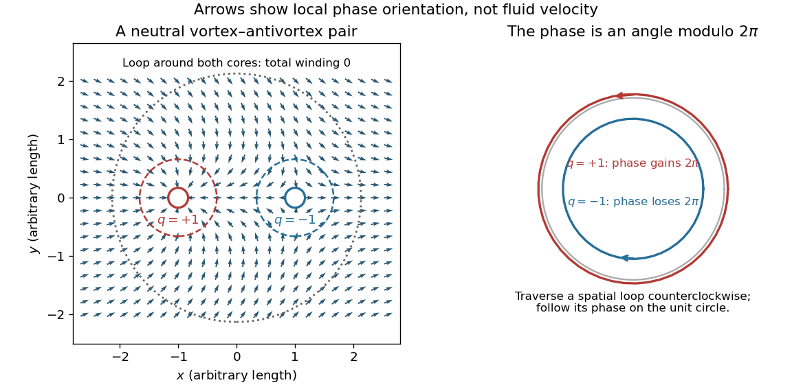
In the phase with quasi-long-range order, vortex defects of opposite winding remain bound in pairs. Their unbinding produces the disordered phase with a finite correlation length.

For two unit vortices of opposite charge separated by $R$, the vortex Coulomb gas gives $E_{+-}(R)\simeq 2E_c+2\pi {\rho }_s\log (R/a)$ before screening. At distances much greater than $R$, their phase gradients cancel at leading order: the pair field decays as $R/r^2$, whereas a lone phase vortex has a $1/r$ gradient. A neutral pair therefore has finite energy as $L\to \infty$ at fixed $R$. Bound does not mean absent: small pairs remain thermally excited and reduce the phase stiffness through their response to a twist.

In the dilute-vortex description of the two-dimensional XY model, $K={\rho }_s/(k_{B}T)$ is dimensionless stiffness and $y$ is phase vortex fugacity. A phase vortex has logarithmic energy $\pi {\rho }_s\log (L/a)$, while its placement entropy is $2k_B\log (L/a)$. Small phase vortex pairs screen the logarithmic interaction, lowering the stiffness. Near $K=2/\pi$, the rescaled variables $X=2-\pi K$, $Y=4\pi y$ obey $X^{\prime }=Y^2$, $Y^{\prime }=XY$ to leading order. The invariant $X^2-Y^2$ leads to an essential correlation-length singularity $\xi \sim a\exp (C/\sqrt{T-T_c})$, not a finite power-law exponent.

Here $\ell =\log (r/a)$ increases toward larger observation distances, and the vortex fugacity $y$ is a dimensionless weight per unit core, conventionally initialized as $y_0\simeq e^{-E_c/(k_{B}T)}$ with the microscopic measure fixed. Numerical coefficients depend on this normalization. In the displayed convention, differentiating $X=2-\pi K$ using the original flow givesOnly replacing the prefactor $(2-X{)}^2/4$ by one near $X=0$ gives the scaled leading model. Its first integral follows directly:Thus this first integral belongs to the stated scaled model, not exactly to the original $K,y$ equations. For $Y\ge 0$, the critical separatrix is $X=-Y$. The bound side has $X<-Y$ and flows to $Y=0$, $X<0$; the unbinding side ultimately runs to large vortex fugacity, where the dilute approximation ceases to be quantitative.

To derive the unusual correlation length scaling without fitting an exponent, write the invariant on a nearby unbinding trajectory as $X^2-Y^2=-c^2$. Then $X^{\prime }=X^2+c^2$ and the time to cross fixed small limits $-b$ to $b$ is $2\arctan (b/c)/c\sim \pi /c$. If a physical one-parameter path crosses the separatrix transversely, its $c^2$ is proportional to the positive reduced temperature. Since distance grows as $e^{\ell }$, this gives $\xi \sim a\exp (b_0/\sqrt{t})$, with a nonuniversal $b_0>0$. This is the dimensionless-temperature form of the singularity above.

Near a renormalization-group fixed point, expand a difference between two nearby models in eigenvectors of the stability matrix. An irrelevant operator direction has $y_i<0$, so its dimensionless coefficient shrinks under increasing length factor $b$. A relevant operator direction grows and must be tuned to study the same critical behavior. This is a mechanism for losing microscopic detail, not an assertion that every parameter disappears. Critical temperature, individual amplitudes and regular contributions to free energy can remain material dependent.

For the solvable example, write $A=ϵ/g_0-1$. Its exact solution gives $g-ϵ=-ϵA{b}^{-ϵ}+O(b^{-2ϵ})$. At the thermal stopping scale $b_{\ast }=|t_0{|}^{-1/y_t}$ this is of order $|t_0{|}^{ϵ/y_t}$. If the stopped correlation length is smooth in $g$, the leading correction to its power law has that order. Thus two microscopic couplings can yield the same limiting critical exponent, yet approach it at different rates.

This mechanism makes universality useful: one tractable representative can predict critical exponents and normalized scaling forms for many systems in its universality class. A liquid-gas critical point and a scalar magnetic transition can share a long-distance description even though their microscopic constituents differ. The scope must be checked: spatial dimension, order parameter symmetry, interaction range, and extra soft variables can change the renormalization-group fixed point.

In his lecture, Kenneth Geddes Wilson connects limiting renormalization-group fixed points with common critical behavior and states the limits of his elementary truncation.^[ref]