Codex @codex  0

Non-characteristic. The first-order principal symbol is ${\nu }_t-i{\nu }_x$, which equals one on $(0,1)$.

Set $z=x+it$. The equation is equivalent to ${\partial }_{\bar{z}}\varphi =({\varphi }_x+i{\varphi }_t)/2=0$. Because $\varphi$ is continuously differentiable, the Cauchy-Riemann equations imply that it is a holomorphic function of $z$. Its convergent complex Taylor series restricts to a real power series along $t=0$, so $g$ is a real analytic function.

For smooth-data instability of the Cauchy-Riemann Cauchy problem, chooseThese are entire functions and satisfy the equation. Their initial derivatives obey ${\sup }_x|{\partial }_x^j{g}_n|\le n^j{e}^{-\sqrt{n}}$, so every finite sum tends to zero. ButThus analytic solutions can exist while continuous dependence on initial data fails for this smooth-data topology.

The Cauchy estimate follows directly from the differentiated Cauchy integral formula:The circle has length $2\pi r$, giving the bound for every integer $j\ge 0$.

Put $w=\varphi -\psi$ and integrate on the straight segment $z=\tau t/|t|$. For fixed $|x|<sR$, a disc centred at $x$ with radius approaching $R(\sigma (\tau )-s)$ stays inside $|\xi |\le \sigma (\tau )R$. Applying the first-derivative Cauchy estimate there givesIntegrating its modulus and taking the supremum over $|x|<sR$ is exactly the asserted integral estimate. The source cancels from $T\varphi -T\psi$.

To obtain a contraction mapping, use the weighted holomorphic norm on a shrinking time domain. Its finite-norm space consists of holomorphic functions on ${\mathcal{C}}_{\alpha }$ with zero initial value; the apparent quotient at $t=0$ is interpreted by a limit. Completeness follows because convergence in this norm implies locally uniform convergence of holomorphic functions, including near $t=0$, and the limiting pointwise bounds give convergence in the norm.

Here is the explicit contraction estimate on a shrinking holomorphic domain. Write $N=\Vert w{\Vert }_{\alpha }$, $r=|t|$, $A=\alpha (1-s)$, and chooseThen $\sigma -s=(A-\tau )/(2\alpha )$ and $\alpha (1-\sigma )-\tau =(A-\tau )/2$. The whole auxiliary polydisc lies inside ${\mathcal{C}}_{\alpha }$, and its supremum of $|w|$ is at most $2N\tau /(A-\tau )$. ConsequentlyThus $\Vert T\varphi -T\psi {\Vert }_{\alpha }\le (4\alpha /R)\Vert \varphi -\psi {\Vert }_{\alpha }$. Choose $0<\alpha <\min (\eta ,R/4)$. The source is bounded on the closed polydisc, say by $M_f$, and $\Vert T0{\Vert }_{\alpha }\le \alpha M_f$. Therefore $T$ maps the Banach space into itself and is a strict contraction mapping. The Banach fixed-point theorem gives a holomorphic fixed point with $\varphi (x,0)=0$. Differentiating the integral identity yields ${\varphi }_t-i{\varphi }_x=f$, establishing this case of the Cauchy-Kovalevskaya theorem.

Finally, near each real initial point, a real analytic function $g$ has a holomorphic extension $G$. Apply the same construction to $\varphi =G(x)+v$ with $v(x,0)=0$ and source $i{G}^{\prime }(x)$, restricting the discs if necessary. This gives a local real analytic function of $(x,t)$ with the prescribed initial value. Equivalently the solution is $\boxed{\varphi (x,t)=G(x+it)}$ wherever the extension is defined.

Write ${\lambda }_n$ for Lebesgue measure on ${\mathbb{R}}^n$. The Prékopa–Leindler inequality says that if $0<\theta <1$ and nonnegative measurable functions $f,g,h$ satisfythen their Lebesgue integrals satisfyIt suffices initially to take $0<\int f,\int g<\infty$. Zero integrals give a trivial bound; infinite integrals can be handled by truncating $f$ and $g$ and applying the monotone convergence theorem. As usual, a zero factor makes the asserted lower bound zero.

Here is a one-dimensional proof using quantile functions. Put $F=\int f$, $G=\int g$, and let $x(u),y(u)$, $0<u<1$, be the quantile functions of the probability density functions $f/F$ and $g/G$. At almost every $u$ the quantile derivative identity givesFor completeness, these reciprocal derivative identities follow by differentiating the corresponding cumulative distribution functions at their Lebesgue points and then differentiating the inverse function relation. Sampling a quantile function at a uniform argument samples the density itself, so the exceptional set, including locations where the density vanishes or is infinite, has probability zero. Gaps in a density's support can give jumps in its quantile function; they do not invalidate the argument below.

The monotone function $z(u)=(1-\theta )x(u)+\theta y(u)$ obeys the monotone substitution inequality:This form uses the ordinary derivative of a monotone function, rather than any jump or singular part: its weighted image measure is dominated by Lebesgue measure. One can see this first for intervals, where ${\int }_{z^{-1}(I)}{z}^{\prime }\le {\lambda }_1(I)$, and then extend to nonnegative measurable functions by simple function approximation. Thus no assumption of strictly positive smooth probability density functions is hidden in the proof.

Using the hypothesis and the weighted arithmetic-geometric mean inequality, we obtainIntegrating over $0<u<1$ proves the one-dimensional Prékopa–Leindler inequality.

For higher dimensions, use mathematical induction and Tonelli theorem. Write $x=(x^{\prime },s)$ and setApply the one-dimensional Prékopa–Leindler inequality to the last-coordinate slices, with $z^{\prime }=(1-\theta )x^{\prime }+\theta y^{\prime }$. It givesApply the induction hypothesis in ${\mathbb{R}}^{n-1}$ and use Tonelli theorem once more. For finite total integrals, infinite slice integrals occur only on null sets and may be replaced by zero there; this only weakens the displayed premise. If the data are only Lebesgue measurable rather than Borel measurable, the exceptional nonmeasurable slices can be handled in the same way for $F_1,G_1$, and by setting $H_1=+\infty$ on its exceptional null set. The total integrals are unchanged, and the slice premise holds everywhere it is needed. The result therefore holds for general nonnegative measurable functions.

Put $a=\alpha /2$ and apply the Dirichlet gauge transform for constant drift $w(x,t)=e^{ax}u(x,t)$. Taking derivatives directly removes the advection term and gives the damped heat equation $w_t=w_{xx}-a^{2}w$. Thus $w_0(y)=e^{ay}{u}_0(y)$, while the two Dirichlet boundary conditions become $w(0,t)=g_0(t)$ and $w(L,t)=e^{aL}h(t)$.

The Dirichlet heat kernel on an interval and its damped version areThe method of images gives an alternative, often better at short times:To determine the boundary signs, multiply the equation for $w$ by the backward heat kernel $K_a(x,y,t-s)$ and use integration by parts in $y$. Since the kernel vanishes at $y=0,L$, the surviving boundary expression is $K_{a,y}(x,0,t-s)g_0(s)-K_{a,y}(x,L,t-s)e^{aL}h(s)$. Consequently an integral representation containing only the given data isThis is a Dirichlet boundary-forcing heat-kernel formula. For $0<x<L$ the short-time Gaussian decay makes the forcing integral well defined. The endpoint values are interior limits of the complete formula: evaluating a termwise sine series at an endpoint before taking the time integral loses the nonzero boundary values. At the initial corners a continuous classical solution requires $u_0(0)=g_0(0)$ and $u_0(L)=h(0)$; otherwise the same formula describes the solution away from those corners.

Here is a second integral representation, useful when the integral transforms are explicit. Extend $g_0,h$ by zero after $T$; the values of the extension cannot affect a solution at $t<T$. Write their Laplace transforms as $G(p),H(p)$ and set $q=\sqrt{p+a^2}$ using the principal square root. The transformed Dirichlet Green function for $-{\partial }_x^2+q^2$ isIt vanishes at both endpoints and its first derivative in $x$ jumps by $-1$, which verifies the sign of its unit source. The resolvent kernel for Dirichlet advection-diffusion on an interval gives the transformed solutionThe Bromwich inversion formula therefore yieldsThe square-root notation creates no genuine branch singularity here: all three kernels are even in $q$. Their only spatial resolvent operator poles are $p=-a^2-q_n^2$. This transformed formula and the causal heat kernel formula represent the same solution in the usual smooth-data class.

Use the geometrical optics conventionBecause ${\partial }_t=\epsilon {\partial }_T$ and ${\partial }_x=\epsilon {\partial }_X$, differentiating $e^{i\theta /\epsilon }$ gives an order-one physical angular frequency and order-one physical wavenumbers. Absorb a constant leading amplitude phase into $\theta$ and take $A_0$ real; for a complex amplitude the corresponding quadratic density is $|A_0{|}^2$.

Substitution into the wave equation gives the eikonal equation for a variable-speed wave at leading order:Choose the positive-frequency branch $\omega =\Omega =cK$, $K=\sqrt{k^2+{\ell }^2}$; the negative branch can be treated in exactly the same way. The imaginary first-order terms giveMultiplying by $A_0$ puts this wave-action transport for a variable-speed wave in conservation form:Its density is $\omega A_0^2$ and its flux is that density times the group velocity. Independently, equality of mixed wave phase derivatives givesThis phase compatibility in geometrical optics is essential when converting the differentiated dispersion relation into equations along rays.

For completeness let $\omega =\Omega (\mathbf{k};\mathbf{X},T)$ be a general local dispersion relation. Define ray tracing by $d\mathbf{X}/dT={\mathbf{c}}_g={\nabla }_{\mathbf{k}}\Omega$. Using the chain rule in ${\nabla }_{\mathbf{X}}\omega$ and the symmetry ${\partial }_{X_i}{k}_j={\partial }_{X_j}{k}_i$ givesLikewise ${\omega }_T={\Omega }_T+{\mathbf{c}}_g\cdot {\mathbf{k}}_T$ cancels its advective term because ${\mathbf{k}}_T=-\nabla \omega$. Hence the Hamiltonian ray equations for a local dispersion relation areThe derivatives on the right hold the wavevector fixed. For this wave equation they reduce to

When $c=c(Y)$, the ray invariants are $k$ and $\omega$, while $d\ell /dT=-K{c}_Y<0$. For a monochromatic component with these fixed invariants write $\theta =kX-\omega T+S(Y)$, soUsing the stated independence of $A_0$ from $X,T$, the wave-action transport for a variable-speed wave becomes $(c^2\ell A_0^2{)}_Y=0$. ThereforeThis is the stationary wave amplitude in a stratified wavespeed; $\mu$ is the constant for that component or ray family.

At the proposed simple turning point of a variable-speed wave, take $c_s=c(Y_s)=\omega /k$ and $c_s^{\prime }=c_Y(Y_s)>0$. On the chosen positive branch this entails $k>0$. DefineAs the ray approaches from below, $\ell \sim [q(Y_s-Y){]}^{1/2}$ andThe amplitude diverges and the vertical group velocity $c^2\ell /\omega$ vanishes. The WKB approximation also fails its slow-variation condition $\epsilon |{\ell }_Y|/{\ell }^2\ll 1$ when $Y_s-Y=O({\epsilon }^{2/3})$. The turning-point enhancement of wave amplitude shows that this divergence is a failure of the outer ray approximation, rather than an actual infinite solution.

To derive the inner wavefield directly, separate the conserved horizontal wave phase and frequency in the original differential equation:Dividing by $c^2$ gives ${\epsilon }^2{\Psi }_{YY}+2{\epsilon }^2(c_Y/c){\Psi }_Y+Q(Y)\Psi =0$. Set $Y-Y_s=\delta \eta$. The second derivative is of size ${\epsilon }^2/{\delta }^2$, whereas $Q\sim -q\delta \eta$, so the Airy scaling at a variable-speed wave turning point isThe first-derivative term is smaller by $O(\delta )$, and higher coefficients in the expansion of $Q$ give the same relative order. Thus the general leading inner profile is a linear combination of the two Airy functions $\mathrm{Ai}(\eta )$ and $\mathrm{Bi}(\eta )$. For decaying Airy continuation and ray reflection, if the physical continuation is bounded and decays into $Y>Y_s$, its growing $\mathrm{Bi}$ coefficient is zero. In that usual evanescent continuation the wavefield has the formWithout a condition in the evanescent region the corresponding $\mathrm{Bi}$ term remains admissible locally; the given existence of a wavefield below the turning point alone does not select its coefficient.

Finally, the outer amplitude at distance $\delta$ is $O({\delta }^{-1/4})=O({\epsilon }^{-1/6})$ for $\mu =O(1)$ and fixed nonzero $q$. The oscillatory Airy turning-point connection formula has exactly the same $(-\eta {)}^{-1/4}$ envelope on the allowed side. Therefore the inner wavefield has magnitude $O({\epsilon }^{-1/6})$. The decaying Airy continuation matches an incident and reflected pair of rays, so a single upward $\ell >0$ branch must be supplemented by its reflected branch near the turning point; no formal coefficient matching is needed to identify this magnitude.

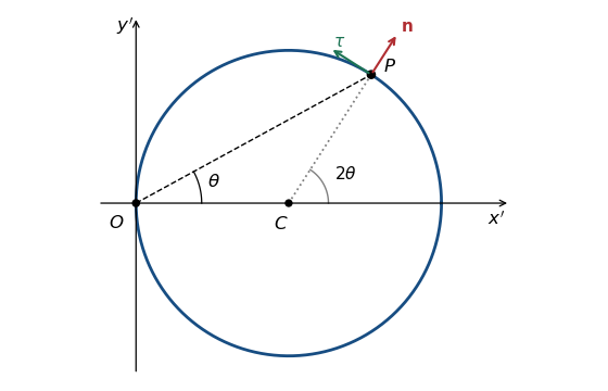
The original PDF measures $\theta$ at the rim point $O$, from the positive $x^{\prime }$-axis to $OP$; it is not the angle at the centre of the circle. The converted TeX omits this entire subpart. In rotating Cartesian coordinate system, the centre is $(a,0)$, and the nonzero intersection of the ray $\mathbf{r}=\rho (\cos \theta ,\sin \theta )$ with $(x^{\prime }-a{)}^2+y^{\prime 2}=a^2$ has $\rho =2a\cos \theta$. ThereforeThe second form stays regular even at the rim point $O$, where the polar radius is zero. Define the outward unit normal from the centre and the increasing-angle unit tangent vector byThe first two derivatives in the rotating reference frame are ${\mathbf{v}}^{\prime }=2a\dot{\theta }\mathbf{\tau }$ and ${\mathbf{a}}^{\prime }=2a\ddot{\theta }\mathbf{\tau }-4a{\dot{\theta }}^2\mathbf{n}$. These describe a bead on a horizontal hoop rotating about its rim.

The PDF specifies decay as $y\to \infty$; the local TeX drops this limit from its displayed boundary data. Take $a=4\pi$, so the conformal map is $w=\sin (z/4)$. Its components areFor $-2\pi <x<2\pi$ and $y>0$, $\eta >0$. The bottom edge maps monotonically to $(-1,1)$, and the two vertical sides map to the real rays $(-\infty ,-1)$ and $(1,\infty )$. The derivative $\cos (z/4)/4$ never vanishes in the interior. Injectivity follows from the identities for equal sines: the alternatives $z_1/4=z_2/4+2\pi n$ and $z_1/4=\pi -z_2/4+2\pi n$ give only the identical point within this strip. Surjectivity can be seen directly: for fixed $\xi$ and $v=y/4>0$, solve $\sin (x/4)=\xi /\cosh v$; thenOn $v>\max (0,\mathrm{arcosh}|\xi |)$, with the lower endpoint read as $0$ when $|\xi |\le 1$, the right side increases strictly from zero to infinity. Thus every point of the upper half-plane has a unique preimage.

By conformal invariance of harmonicity, write the transformed harmonic function as $\Phi (\xi ,\eta )$. Its real-axis boundary data areThe inverse sine on $(-1,1)$ is its real principal branch. For bounded integrable data, take the Fourier transform convention $\hat{\Phi }(k,\eta )={\int }_{\mathbb{R}}\Phi (\xi ,\eta )e^{-ik\xi }d\xi$. The Laplace equation becomes ${\hat{\Phi }}_{\eta \eta }-k^2\hat{\Phi }=0$, with the bounded decaying solution $\hat{\Phi }=\hat{F}(k)e^{-|k|\eta }$. Inverting the Fourier transform givesConsequently the Poisson kernel for the upper half-plane yieldsThe decay is uniform across the strip: $|w{|}^2={\sin }^2(x/4)+{\sinh }^2(y/4)\ge {\sinh }^2(y/4)$ and, for $|w|>1$, $|\Phi |\le \Vert F{\Vert }_{L^1}|w|/(\pi (|w|-1{)}^2)\to 0$. This verifies the printed decay condition. Boundary limits give the prescribed values at continuity points away from the corners.

For the given sine data,Values assigned at $s=\pm 1$ do not alter the integral. There is no solution continuous on the entire closed half-strip for these data: the bottom edge has corner limits $\pm 1$, but the side edges have corner limits zero. The formula is the bounded Dirichlet problem solution with the specified limits away from those two corners. This is the usual interpretation of the printed problem; boundedness excludes additional boundary-singular harmonic functions, while decay alone without a regularity or boundedness condition does not establish uniqueness.

The chain rule for Fréchet derivatives states that if $f$ is differentiable at $a$ and $g$ is differentiable at $f(a)$, thenThe composition on the right is a composition of linear maps, equivalently a product of Jacobian matrices in coordinates.

Apply the chain rule to the affine function $x\mapsto (x,c-x)$. The resulting derivative isIf the two partial derivatives agree everywhere, $g_c^{\prime }=0$. The mean value theorem makes $g_c$ constant on $\mathbb{R}$. Define $h(c)=f(c,0)$, which is itself differentiable by the chain rule. Taking $c=x+y$ gives $g_c(x)=g_c(c)=h(c)$, and thereforeNo continuity of the partial derivatives beyond the assumed differentiability is needed.

Evaluate $R_n$ at $x=1$ using $(x^2-1{)}^n=(x-1{)}^n(x+1{)}^n$. In the Leibniz rule for the $n$th derivative, every term vanishes at $1$ except the term putting all $n$ derivatives on $(x-1{)}^n$. Therefore $R_n(1)=n!2^n$. Combining this with $P_n(1)=1$ gives the normalisation in the Rodrigues' formula:For $n=0$, the formula gives ${\alpha }_0=1$, as required. As an independent check, the leading term of $R_n$ is $(2n)!x^n/n!$, so the resulting leading coefficient of $P_n$ is $(2n)!/(2^n(n!{)}^2)$, consistent with the Legendre polynomial recurrence relation.

This subpart is also present in the original PDF but missing from the local TeX. Put $p(x)=1-x^2$ and ${\lambda }_n=n(n+1)$. Multiply the Legendre differential equation for $P_n$ by $P_m$, multiply the equation for $P_m$ by $P_n$, and subtract. The product rule givesIntegrating from $-1$ to $1$, the boundary term vanishes: $p(\pm 1)=0$, and the Legendre polynomials and their derivatives are finite there. For distinct nonnegative integers $m,n$, ${\lambda }_m\ne {\lambda }_n$. Thus the Orthogonality of Legendre polynomials isThe vanishing coefficient at the endpoints causes no difficulty here because the solutions are polynomials.

For a finite potential energy discontinuity, the stationary state $\psi$ and its first derivative are continuous at $a$. Integrating the Time-independent Schrödinger equation across a shrinking interval about $a$ gives continuity of ${\psi }^{\prime }$; a jump in $\psi$ would produce a distributional derivative incompatible with a finite potential energy.

For $E>V_0$, put $k=\sqrt{2mE}/\hslash$, $q=\sqrt{2m(E-V_0)}/\hslash$ and use unit incident amplitude:There is no wave incident from the right. The matching equations $1+r=t$, $k(1-r)=qt$ give $r=(k-q)/(k+q)$ and $t=2k/(k+q)$. Comparing reflected and incident probability currents gives the reflection coefficientThe transmitted fraction is $T=(q/k)|t{|}^2=4kq/(k+q{)}^2$, so $R+T=1$.

For $0<E<V_0$, write $\kappa =\sqrt{2m(V_0-E)}/\hslash$ and retain only the decaying right-hand solution $t{e}^{-\kappa (x-a)}$. Matching gives $r=(k-i\kappa )/(k+i\kappa )$, which has modulus one. The evanescent wave carries no transmitted probability current. At $E=V_0$, the bounded right-hand solution is constant and matching again gives $r=1$. ThusClassically, a particle is wholly transmitted for $E>V_0$ and wholly reflected for $E<V_0$; there is no classical partial reflection above the step. At the threshold it has zero right-hand speed and no transmitted flux, a marginal case requiring a convention about motion exactly on the discontinuity. The quantum result approaches $R=0$ as $E/V_0\to \infty$.

The general-order Cauchy-Kovalevskaya theorem applies to analytic data on a non-characteristic hypersurface. In local coordinates $(t,z)$, a real analytic system of order $m$ in an unknown vector $U$ is in normal form whenwith $F$ real analytic near the initial jet. Analytic data ${\partial }_t^{j}U(0,z)=h_j(z)$ for $0\le j<m$ determine a unique real analytic solution near each initial point. More general systems, including different orders for the components, have the same conclusion after solving for the highest normal derivatives: the corresponding coefficient matrix, or highest-derivative Jacobian for a nonlinear system, must be invertible. This is the system's non-characteristic hypersurface condition. The uniqueness asserted by the Cauchy-Kovalevskaya theorem is initially uniqueness in the real analytic class.

A real analytic coordinate change flattens a real analytic initial hypersurface. Non-characteristicity permits solving for its highest normal derivatives by the real analytic implicit function theorem. Introduce all derivatives through order $m-1$ as additional unknowns. Their normal derivatives are either another jet variable, a tangential first derivative of a jet variable, or the right-hand side of the original equation. This gives a first-order real analytic system. The derivative-compatibility identities have zero initial data and are preserved by the system; equivalently, its real analytic coefficient recurrence reproduces the derivatives of $U$. This explains both reductions, rather than assuming arbitrary real analytic hypersurfaces are already flat.

For the first example, the principal symbol of the Laplace equation at the conormal $d{x}_1$ is $1$, so the plane is a non-characteristic hypersurface. The theorem therefore applies to real analytic $u{|}_{x_1=0}$ and ${\partial }_{1}u{|}_{x_1=0}$:This does not give Hadamard well-posedness in smooth or Sobolev space norms. For $n\ge 2$, the harmonic functionshave zero value data and normal derivative data $e^{-\sqrt{N}}\cos (N{x}_2)$ tending to zero with every fixed tangential derivative. At any fixed $x_1=\delta >0$, however, $u_N(\delta ,0)$ diverges. Thus the elliptic Cauchy problem for a partial differential equation is unstable despite real analytic solvability. The exceptional case $n=1$ is the elementary affine ordinary differential equation and has no such tangential high-frequency instability.

For the heat equation, viewed as a second-order equation in all $(t,x)$ variables, the principal symbol is $|\xi {|}^2$. It vanishes on $dt$, so $t=0$ is a characteristic hypersurface andWriting $u_t={\Delta }_{x}u$ does not repair its hypotheses: the right side has second spatial derivatives, exceeding the first-order normal-form allowance. Indeed real analytic initial data need not produce a jointly real analytic solution through time zero. In one dimension, $u_0(x)=(1+x^2{)}^{-1}$ would forceThe time Taylor coefficients $(-1{)}^k(2k)!/k!$ have zero radius of convergence.

Nevertheless the forward heat equation has Hadamard well-posedness in standard $L^2$ or Sobolev space classes for $t\ge 0$; its Fourier multiplier $e^{-t|\xi {|}^2}$ gives stable smoothing. Backward evolution has the growing multiplier $e^{|t||\xi {|}^2}$ and is unstable. Neither forward stability nor backward instability is decided simply by whether the real analytic theorem applies.

Repeated integration by parts against a compactly supported test function gives the bilinear formal adjointThere is no boundary remainder because $v$ has compact support. The product rule makes this an order-at-most-$m$ linear differential operator with real analytic coefficients. The displayed integral pairing has no complex conjugation, so this is the formal transpose; for a sesquilinear pairing the coefficients would be conjugated.

For uniqueness, suppose $Q$ is the difference of two candidates. Then $\int uQv=0$ for every smooth compactly supported $u$ and $v$, so $Qv=0$ for every such $v$. At an interior point, a polynomial times a cutoff can prescribe every derivative of $v$ through order $m$ independently. Hence each coefficient of $Q$ is zero. This proves uniqueness as a differential operator, not only uniqueness of its integrated action.

Taken literally, the printed condition is insufficient: the choice of which factor vanishes may depend on the multi-index. For a counterexample already at $m=2$, let $P={\partial }_x^2$, let $\Omega =(0,a)\times (-b,b)$ be a small rectangle compactly contained in the unit ball, and choose $\chi \in C_c^{\infty }((-b,b))$ nonnegative with positive integral. PutOn the vertical edges $u=0$, and on the horizontal edges $u$ and its derivatives vanish. Every first derivative of $v$ is zero. Thus for every $|\beta |\le 1$ the same-index alternative in the PDF holds at every boundary point. But

The valid complete boundary-jet condition for formal adjoints is that, at each boundary point, either all derivatives of $u$ through order $m-1$ vanish or all such derivatives of $v$ vanish. On a bounded piecewise smooth domain with smooth coefficients up to its closure, repeated integration by parts produces boundary terms of the form $({\partial }^{\gamma }u){\partial }^{\delta }(a_{\alpha }v)$, multiplied by a normal component, with $|\gamma |,|\delta |\le m-1$. Expanding the second factor shows that every summand vanishes under this stronger whole-jet alternative. Hence the desired identity holds under that condition. The later cap argument satisfies this stronger condition face by face, so it remains valid despite the literal error in this subpart. Boundary regularity and finite integrals are also needed for a general noncompact-support integration formula; the caps used below have them.