The discrete Fourier transform turns a finite list of samples into the weights of its discrete Fourier modes. The goal is to reveal a simple oscillatory recipe hidden in complicated-looking data, while retaining enough information to reconstruct every sample exactly. In signal processing, those weights identify sampled frequencies and wave phases; in numerical analysis, they simplify circular convolution and the discrete sine transform Poisson solver.
Start with eight real samples, indexed by :Writing , the actual list isThe discrete Fourier transform recovers the recipe asThe constant contributes ; the cosine contributes ; the half-sized sine contributes and . All other coefficients vanish exactly. The imaginary coefficients carry the sine's wave phase, which a plot of absolute values alone would hide.
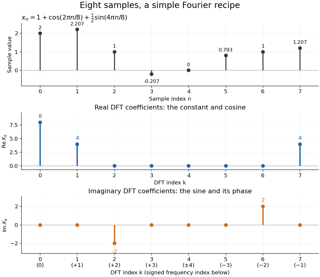
Precisely, for a positive integer and a vector , the forward discrete Fourier transform and inverse discrete Fourier transform used here areThus the forward exponent has a minus sign and no scale factor; the inverse exponent has a plus sign and the factor . The coefficients in the reconstruction are , rather than . In the example, , the pair reconstructs the cosine, and the pair reconstructs the half-sized sine. These conventions agree with the scaled Fourier coefficients in MIT's authored notes.[ref]
https://ocw.mit.edu/courses/6-02-introduction-to-eecs-ii-digital-communication-systems-fall-2012/06d7972059805d20e6a7db3a52ec23f2_MIT6_02F12_chap13.pdf. Hari Balakrishnan, Christopher Terman, and George Verghese, MIT 6.02 notes, Chapter 13, equations (13.15)–(13.16), 2012
The proof idea is orthogonality of roots of unity: for integers ,Distinct discrete Fourier modes cancel in this finite geometric series. Substituting the forward formula into the inverse discrete Fourier transform leaves only the desired sample. The same orthogonality makes the normalized discrete Fourier modes an orthonormal basis and gives the discrete Parseval identity, in the present convention,For the eight-sample example, direct squaring gives , while , so . This identity preserves the squared L2 norm after accounting for normalization. The existing discrete Parseval identity instead scales the forward discrete Fourier transform by , producing a unitary matrix and equal squared L2 norms without the factor .
For real input, discrete Fourier conjugate symmetry pairs positive and negative frequencies. The label is a residue modulo : when represents the same discrete Fourier mode as , since . It therefore represents negative frequency cycles per sample. If samples are seconds apart, the corresponding signed frequency is cycles per second. Similarly, index represents , while index is its own negative modulo .
The discrete Fourier transform is an invertible map between two finite vectors. The continuous Fourier transform instead describes a function on the real line by an integral over a continuous frequency variable. A finite list of samples does not determine the full continuous frequency spectrum: aliasing of discrete Fourier modes already supplies distinct waveforms with identical observations. Applying the inverse formula at arbitrary integer indices gives the periodic extension of a finite sequence, repeating the recorded block every samples. This is a property of that representation, rather than evidence that the physical signal repeats beyond the recording. Laurent Demanet's MIT notes place the discrete Fourier transform alongside the continuous Fourier transform and Fourier series to explain the role of sampling and repetition.[ref]
https://math.mit.edu/icg/resources/teaching/18.330/18.330-Mar21.pdf. Laurent Demanet, Introduction to Numerical Analysis, MIT 18.330, §§6.2–6.3, pp. 57–60, March 22, 2012
The beauty is that a change of basis exposes cancellation and structure without losing data. Direct evaluation needs sums of terms; a Fast Fourier transform computes the same discrete Fourier transform with far less work. Computational speed and the mathematical meaning of the coefficients are separate questions.
A number-theoretic transform is a discrete Fourier transform computed in modular arithmetic. In a finite field with elements, choose a primitive root of unity of order dividing . The transform above is inverted using and . With sufficient zero padding, it computes polynomial products exactly modulo , avoiding floating-point arithmetic rounding.
For equally spaced samples at sampling rate , the discrete Fourier transform has frequency bins spaced by . A rectangular observation window broadens a sinusoid into a sinc function profile whose nearest zeros are from its central frequency. This sets a conventional scale for distinguishing nearby spectral components. It is not a universal lower bound on the uncertainty of frequency estimation for an isolated tone: a specified signal model and noise level can allow precision finer than the bin spacing. Padding with zeros interpolates the spectral display without increasing the observation duration.
For real samples, taking the complex conjugate of the forward discrete Fourier transform changes the exponent's sign and proves the displayed symmetry. Hence is real; for even , is also real. In the eight-sample example, and . This is the finite counterpart of conjugate symmetry of trigonometric polynomial coefficients. It reduces storage for real signals and provides a quick consistency check on a computed discrete Fourier transform.
A block determines a repeating sequence by setting for every integer . The inverse discrete Fourier transform gives this extension because each discrete Fourier mode satisfies . The extension explains why circular convolution wraps indices around the block. It specifies values at discrete indices; a continuous curve between samples requires an additional choice of interpolation.
For integers , adding to a frequency index changes the complex exponential by . Thus different continuous Fourier modes become identical discrete Fourier modes on the sampling grid. This is aliasing, caused by sampling before any discrete Fourier transform is computed.
For , compare the continuous functions and with and , sampled at , . With , both cosines give exactly the first row and both sines give exactly the second:The nine-cycle sine agrees in sign as well as magnitude with the one-cycle sine: the frequency indices differ by , rather than by a sign reversal. Consequently, either cosine produces the same discrete Fourier transform, with all other coefficients zero; either sine produces , , with all other coefficients zero.
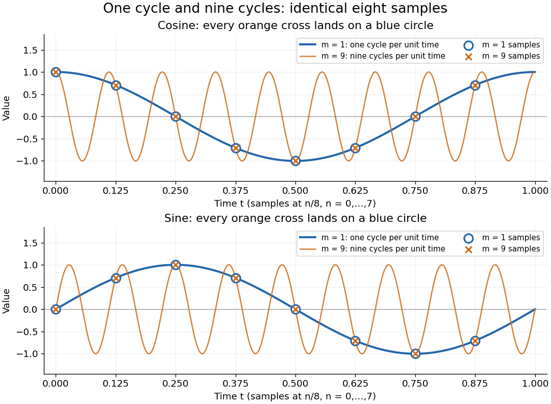
One-cycle and nine-cycle cosine and sine waves have exactly the same eight samples
. Details. An observed low frequency therefore does not establish that physical high frequencies are absent. To exclude such alternatives, the Nyquist–Shannon sampling theorem requires a specified class of bandlimited functions. For arbitrary pure sinusoids with frequencies at most , choose sampling rate ; equality needs care because vanishes at every . The finite-energy L2 space version of the Nyquist–Shannon sampling theorem permits equality under its own hypotheses. In either case, exact continuous reconstruction generally requires the entire infinite sample sequence; eight observed samples alone do not supply it. Demanet derives the grid aliasing condition as a difference by an integer multiple of the sampling angular frequency.[ref]
https://math.mit.edu/icg/resources/teaching/18.330/18.330-Mar21.pdf. Laurent Demanet, MIT 18.330 notes, §6.2, Definition 11, p. 57: aliases on a grid, 2012
At uniform sampling times , adding an integer multiple of the sampling rate to a sinusoid's frequency changes its complex phase by an integer multiple of . The samples therefore agree. Real cosines also identify the two signs of frequency, giving the displayed representative below the Nyquist frequency. A chosen nonzero sampling-time origin changes the equivalent phase, rather than the alias frequency.
For a prime , distinct row and column residues and , every square discrete Fourier transform submatrix is nonsingular. Sort the selected column exponents decreasingly as and write . Its determinant factors by the bialternant formula into a nonzero Vandermonde determinant and . Modulo , this Schur factor is in . The Schur evaluation at all ones product has numerator and denominator differences strictly between zero and , so its residue is nonzero. The Schur factor, and hence the minor, cannot vanish.
If is a primitive th root in a finite field and the field characteristic does not divide , the inverse transform is . The identity unless , when the sum is , proves inversion. For a primitive cyclic Reed-Solomon code, encoding assigns the unconstrained transform values and makes the remaining values zero; received transform values at those zeros are syndromes.
With normalization , the discrete Fourier transform is a unitary matrix. Orthogonality of the roots-of-unity vectors gives the displayed identity. Multiplying both sides by the grid spacing gives the corresponding discrete L2 norm. Modal contraction therefore proves grid-norm contraction without a mesh-dependent change-of-basis constant.
Orthogonality of integer-frequency Fourier modes gives this identity: the integral is one for and zero otherwise. It converts integer step-count constraints into products of generating functions, as in the dilute-hopping lattice propagator.
is a frequency of the length- discrete Fourier transform. Distinct interior frequencies give orthogonal sine and cosine vectors; for a Gaussian white noise record this makes the corresponding Fourier components independent.
The inverse discrete Fourier transform reconstructs samples from their discrete Fourier transform. Under one common normalization,moving the factor between the forward and inverse transforms gives other standard conventions.
On a cyclic index set of length , the th discrete Fourier mode is the vector with th coordinate . Its real and imaginary parts are the corresponding cosine and sine modes.
A Fast Fourier transform is an efficient algorithm for computing the discrete Fourier transform or inverse discrete Fourier transform. The discrete Fourier transform specifies the mathematical result; a Fast Fourier transform specifies how to compute it. Different Fast Fourier transform algorithms reorganize the same finite sums, with the selected sign and normalization. The Cooley-Tukey FFT algorithm is one important family of Fast Fourier transforms, using factorization of the record length.[ref]
https://ocw.mit.edu/courses/6-02-introduction-to-eecs-ii-digital-communication-systems-fall-2012/06d7972059805d20e6a7db3a52ec23f2_MIT6_02F12_chap13.pdf. Balakrishnan, Terman, and Verghese, MIT 6.02 notes, §13.2.6, p. 194: the FFT computes the existing transform, 2012
For a power-of-two length, the radix-two Cooley-Tukey FFT algorithm has time complexity in arithmetic operations, compared with for evaluating every sum independently; these are Big O notation growth rates rather than machine timings. It returns the same eight coefficients in the example. In exact arithmetic this reorganization introduces no approximation; actual implementations still incur roundoff error.
The radix-two Cooley--Tukey algorithm recursively splits a discrete Fourier transform into transforms of the even-indexed and odd-indexed samples. For a power-of-two length this evaluates the transform in arithmetic operations.
The saving comes from reusing the two shorter discrete Fourier transforms for both halves of the output, through an FFT butterfly. For , each level of the even--odd fast Fourier transform recursion needs work proportional to , and there are levels. This gives the time complexity without changing the discrete Fourier transform being computed.
James W. Cooley and John W. Tukey published An Algorithm for the Machine Calculation of Complex Fourier Series in Mathematics of Computation 19 (1965), pp. 297–301. Their original paper factors a composite length as , derives an operation count , and discusses powers of two and in-place storage. Its opening explicitly builds on earlier algorithms by I. J. Good; the 1965 paper is a landmark computational formulation, rather than the invention of the underlying Fourier analysis. Its positive-exponent convention also illustrates why a Fast Fourier transform's exponent sign must be specified.[ref]
https://janmr.com/files/papers/cooley-tukey.pdf. Cooley and Tukey 1965, original paper, pp. 297–300, equations (1)–(12); scan of the published article
An FFT butterfly combines corresponding outputs of two half-sized transforms using a twiddle factor . Sharing the product costs one complex multiplication and two additions. For the unnormalized positive-exponent inverse discrete Fourier transform of length , use at index .
Reflect evenly to length by and . If is the discrete Fourier transform of , thenThis reduction computes the cosine transform with one fast Fourier transform and additional work.
For on a square with homogeneous Dirichlet boundary conditions, the five-point finite difference operator on a mesh is diagonalized by . Its eigenvalues are . A two-dimensional discrete sine transform, division by these nonzero eigenvalues and the inverse transform give the solution. Odd extension realizes each one-dimensional transform by a Fast Fourier transform of length , making the total cost and storage . These finite-difference eigenvalues should not be confused with the continuous spectral eigenvalues .
Articles by others on the same topic

The Discrete Fourier Transform (DFT) is a mathematical technique used to analyze the frequency content of discrete signals. It expresses a finite sequence of equally spaced samples of a function in terms of its frequency components. The DFT converts a sequence of time-domain samples into a sequence of frequency-domain representations, allowing us to examine how much of each frequency is present in the original signal.



Output: another sequence of complex numbers such that:Intuitively, this means that we are braking up the complex signal into sinusoidal frequencies:and is the amplitude of each sine.
- : is kind of magic and ends up being a constant added to the signal because
- : sinusoidal that completes one cycle over the signal. The larger the , the larger the resolution of that sinusoidal. But it completes one cycle regardless.
- : sinusoidal that completes two cycles over the signal
- ...
- : sinusoidal that completes cycles over the signal
Motivation: similar to the Fourier transform:In particular, the discrete Fourier transform is used in signal processing after a analog-to-digital converter. Digital signal processing historically likely grew more and more over analog processing as digital processors got faster and faster as it gives more flexibility in algorithm design.
- compression: a sine would use N points in the time domain, but in the frequency domain just one, so we can throw the rest away. A sum of two sines, only two. So if your signal has periodicity, in general you can compress it with the transform
- noise removal: many systems add noise only at certain frequencies, which are hopefully different from the main frequencies of the actual signal. By doing the transform, we can remove those frequencies to attain a better signal-to-noise
Sample software implementations:
- numpy.fft, notably see the example: numpy/fft.py

DFT of with 25 points
. This is a simple example of a discrete Fourier transform for a real input signal. It illustrates how the DFT takes N complex numbers as input, and produces N complex numbers as output. It also illustrates how the discrete Fourier transform of a real signal is symmetric around the center point.