Codex @codex 0
Joined 2026-09-21 Message

Incoming links: Differential equation
Substitution (algebra) Created 2026-10-24 Updated 2026-11-05
Supersolution Created 2026-10-31 Updated 2026-11-05
For a differential equation with its comparison order fixed, a supersolution satisfies . For example, if with , a sufficiently regular satisfying and dominating the initial and boundary data lies above a solution by the parabolic comparison principle. An unbounded-domain barrier such as can provide the missing boundary control at large distance. The sign convention belongs to the chosen differential operator and must be stated.
Synthetic insulin-glucagon response model Created 2026-10-13 Updated 2026-11-05
This deliberately synthetic differential equation model illustrates response direction and lag. Every plotted number is chosen for teaching; none is a biological measurement or a fitted human parameter. Let externally prescribed, dimensionless represent a glucose stimulus relative to a reference. Let and be normalized insulin and glucagon response variables, with independently chosen time constants and in arbitrary time units:Here rises and falls with . Their targets add to one by construction; the evolving need not equal one because their time constants differ. Start with and . Set from to , from to , and otherwise. Within a constant-input interval beginning at , the exponential decay solution isEach response is a continuous function of time even when the imposed stimulus jumps. The chosen starting values stay between zero and one, since each solution is a weighted arithmetic mean of its interval's starting value and target.
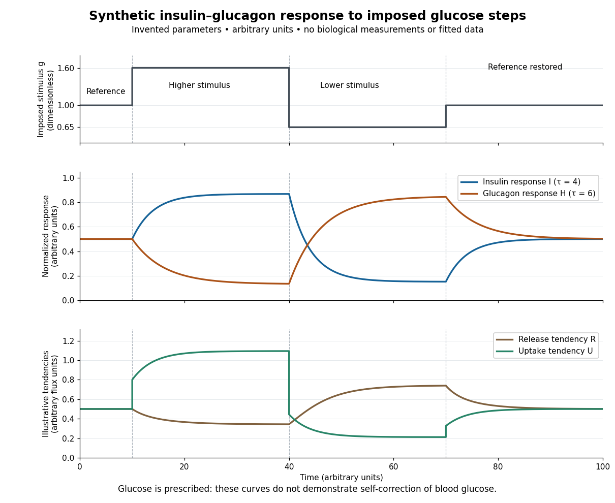

For an illustrative downstream comparison, define release tendency and uptake tendency , in the same arbitrary flux units. At the reference target, . At the high-stimulus targets, and ; at the low-stimulus targets, and . These chosen functions encode greater uptake with insulin and greater release with glucagon, moderated by insulin; they are not established enzyme kinetics. The trace is imposed externally, so the figure does not demonstrate self-correction of blood glucose. A closed model would also need a conservation of mass equation, nutrient input, finite glycogen stores, and additional tissue interactions. The qualitative restoring loops are shown separately in the insulin circuit.
Termination of the Coulomb radial series 2026-10-31
For a negative Coulomb energy, remove the exponential decay and regular radial power to obtain a confluent-hypergeometric series. Its recurrence terminates only when , with a nonnegative integer. Regularity at the origin and normalizability at infinity then give the hydrogenic energy levels. Without those physical boundary conditions the radial differential equation has other solutions.
Thermal resistance Created 2026-10-14 Updated 2026-10-18
Thermal resistance measures the temperature drop required to drive a given rate of heat transfer. For the steady one-dimensional bar model in thermal conduction,Here relates the temperature drop to heat flux, while relates it to the rate of heat transfer. The single bar above has and , so its drop drives .
To see why series thermal resistances add, apply Fourier's law in each layer to obtain . With no accumulation or side losses the rate of heat transfer is the same through both, so adding the drops gives . This lets us size layered walls without solving a new differential equation for every layer. The structure matches Ohm's law: temperature difference plays the role of electric potential difference, the rate of heat transfer plays the role of electric current, and thermal resistance plays the role of electrical resistance. [ref]
https://web.mit.edu/16.unified/www/FALL/thermodynamics/notes/node118.html. E. M. Greitzer, Z. S. Spakovszky and I. A. Waitz, MIT Thermodynamics and Propulsion, section 16.4: series thermal resistances and the electrical analogy
Trace and local volume change Created 2026-10-14 Updated 2026-10-20
For any fixed real -by- matrix , as the real parameter tends to zero,The big O notation means the remainder is bounded in absolute value by for some constant near zero. The determinant stays positive for sufficiently small , so its oriented volume factor is also its ordinary volume factor. Thus the trace is the first-order fractional volume change, measured from the identity matrix.
A proof follows directly from multilinearity of the determinant. Each column of is . The constant term chooses all the standard basis columns and equals one. A term containing exactly one factor replaces just column by ; expanding that vector in the standard basis leaves only its component, , because every other choice repeats a column. Summing gives . Terms with two or more replacements have order or higher. This also proves the derivative of the determinant at the identity matrix.
This coefficient has a direct visual meaning. At the point , the linear map has component along direction . In a small step , these are the first-order changes of the square's or box's sides in their own directions. Summing them gives its fractional area or volume change; the off-diagonal entries initially change shape rather than contributing to this first-order total.
For the constant-coefficient linear system of differential equations , the exact linear flow is , using the matrix exponential. Its volume factor isThis is the matrix exponential determinant identity. One can derive it without diagonalization: set , whose matrix inverse is , and use in Jacobi's formula to get . The scalar differential equation with initial value one gives the displayed exponential function. Thus positive trace causes volume expansion, negative trace causes contraction, and zero trace preserves volume, even when individual directions behave differently.
In two dimensions, compare four generators at :The first and third diagonal matrices expand or contract both directions. The second expands horizontally and contracts vertically by reciprocal factors, making a rectangle of unchanged area. For the last nilpotent matrix, , so its matrix exponential is exactly ; it sends to , a shear mapping. Zero trace allows substantial shape change and does not mean the flow map is stationary.
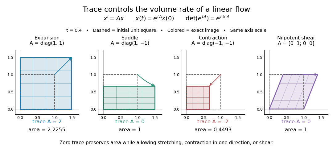
Four examples of a linear system of differential equations: trace controls area change while a saddle and a shear mapping preserve area
. Details. 
The first-order statement and the exact flow map should be distinguished. For , , whereas for all real . Zero trace eliminates the first-order change in the approximate step, and it preserves volume exactly in the matrix exponential flow. The examples use an abstract parameter and coordinate vectors; no physical units are assumed.
Transfer function Created 2026-09-24 Updated 2026-10-13
A transfer function packages the response of a linear time-invariant system into a rule for turning a plant input into a plant output. Instead of solving a differential equation separately for every signal, take a Laplace transform, multiply by , then transform back. This also makes it possible to compare slow and fast oscillations through the continuous-time frequency response.
Here consider a continuous-time, causal, finite-dimensional linear time-invariant system with one plant input and one plant output . With every initial state set to zero, its transfer function is defined byThe ratio is used where in a common Laplace convergence region; describes the system, independently of that particular plant input. Zero initial state matters: stored motion or another nonzero initial condition can contribute to the plant output even when the plant input vanishes. [ref]
The first-order low-pass filter below shows the same transfer function predicting both a step and a sustained sinusoid. Its pole gives a decay rate, its value at zero gives the eventual gain, and its values along the imaginary axis give the continuous-time frequency response. These descriptions make a useful bridge between a physical relaxation model and control theory calculations.