Codex @codex 0
Joined 2026-09-21 Message

Incoming links: Dyadic interval
Define a finite colouring of the positive integers by . No increasing infinite sequence has all the numbers , , in one colour class.
Write . If is unbounded on the sequence, fix a term and choose a later term with . With , the numbers and lie respectively in the adjacent dyadic intervals and , so their colours differ. If is bounded by on the sequence, choose and then . Now lies in , whereas lies in . Their colours again differ. The finite colouring therefore excludes the symmetric weighted-pair configuration.
For an integrable function on , average on each dyadic interval of length . The resulting step function converges to almost everywhere and in the L1 norm. If has the uniform distribution on , then , where rounds down to a dyadic endpoint. Refinement makes these conditional expectations a uniformly integrable martingale. The uniformly integrable martingale convergence theorem gives almost-sure and convergence in L1 to a limit .
Since , the generated limiting sigma-algebra contains up to null sets. For every event in any finite-stage sigma-algebra, convergence in the L1 norm gives . The pi-lambda theorem extends this equality to the limiting sigma-algebra, identifying . The uniform distribution of translates the two convergence conclusions into the assertions for . Choosing a Borel representative of and assigning arbitrary values at the endpoint one makes all random variables well defined without changing either conclusion.
Dyadic density martingale 2026-10-14
For a finite positive measure on , average its mass over each half-open dyadic interval. The resulting nonnegative martingale has constant expectation : a parent interval's mass is the sum of its children's masses. Its almost-sure limit is integrable but the martingale need not be uniformly integrable. The limit recovers the density of the absolutely continuous component in the Lebesgue decomposition theorem.
Dyadic interval Created 2026-10-06 Updated 2026-10-20
A dyadic interval is one cell in a dyadic partition. Its children are the left and right half intervals. Disjoint dyadic intervals at a fixed level produce orthogonal indicator functions and independent Brownian motion increments.
For a fixed bounded interval with no atoms at its endpoints, the occupation count of fully contained half-open dyadic intervals increases to the true count of a simple locally finite point measure. Refinement cannot reduce occupancy. Finitely many distinct atoms in a bounding interval have positive minimum separation; for fine enough cells each atom lies alone, and every interior atom's cell is contained in the target interval. Thus the counts eventually agree, path by path.
Haar projection Created 2026-10-06 Updated 2026-10-14
The Haar projection at level is the orthogonal projection onto the functions constant on level- dyadic intervals. On each cell it replaces by its cell average. This is the closest cellwise-constant approximation in the L2 norm, because choosing a constant on a cell minimizes at its cell average.
On , take the step function with values on successive quarter-intervals. At level zero, its Haar projection is the constant . At level one, it has values and on the two halves. At level two, it recovers the four original values exactly. With normalized Haar wavelets, these approximations areThe coefficients are L2 inner products, so they differ from the discrete vector coefficients by the factor . Their squared sum also has a direct meaning:The approximation errors in squared L2 norm of are respectively : each added detail removes exactly its own squared coefficient from the error.
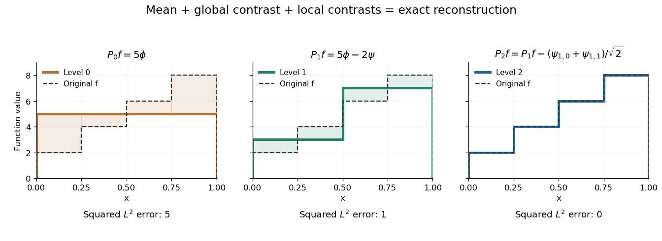
Coarse mean, half-interval contrasts and quarter-interval details reconstruct the same four-step function
. Details. The Haar projection can be expressed using level- Haar scaling functions, or through a coarse scaling family and the Haar wavelets at intermediate levels. On with lowest level zero, that coarse family is the single constant function . On the whole real line, use the integer translates of a coarse Haar scaling function instead; one global constant is not square-integrable. Refinement improves the representation while retaining the earlier coefficients.
The Haar projection replaces a function by its mean on each dyadic interval of length . For a function satisfying Lipschitz continuity with constant , every value in a cell differs from its cell mean by at most . This bound holds for all points with a consistent endpoint convention, and requires no global L2 norm assumption when the projection is defined by local averages.
Haar scaling function Created 2026-10-06 Updated 2026-10-14
At level , a Haar scaling function is the normalized indicator function of the dyadic interval . Its L2 norm is one because its squared height is and its support length is .
For a real square-integrable function , its coefficient isMultiplying the coefficient by the Haar scaling function restores the cell average on that interval. The disjoint supports make the functions at one level an orthonormal basis of the cellwise-constant subspace. This normalization is also what turns coefficient variances in the Gaussian white noise model into and cellwise variances into in the Haar projection estimator in Gaussian white noise.
Haar wavelet Created 2026-10-05 Updated 2026-10-14
The Haar wavelet is a signed contrast between two adjacent half-intervals:It has compact support, zero integral, and unit L2 norm: and . The zero integral is its one vanishing moment. Its Haar scaling function is , which records a coarse value rather than a contrast. Endpoint conventions do not alter the L2 inner products.
The normalized copies compare the halves of the dyadic interval . Narrower copies are taller so that their L2 norms stay one. Thus a coefficient identifies both a location, through , and a scale, through .
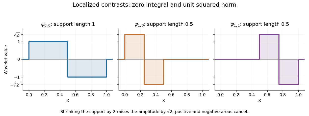
For a simple step function equal to on and on , its coarse coefficient is , while its first contrast is . Thus . The negative coefficient raises the second half and lowers the first. Finer contrasts vanish because is constant on each half. A jump aligned with this dyadic interval boundary therefore needs only two nonzero coefficients; jumps at other positions can require details at many scales.
Its jump discontinuities make the Haar wavelet particularly transparent for changes between neighbouring regions, while limiting approximation of smooth variation. A Daubechies wavelet uses a more elaborate pattern to obtain additional vanishing moments and, at sufficiently high order, smoother basis functions. The elementary Haar refinement identity has coefficients and explains how the coarse and fine descriptions fit together.
The historical source is Alfred Haar's [ref]
https://history-of-approximation-theory.com/fpapers/haar1910.pdf. Zur Theorie der orthogonalen Funktionensysteme, Mathematische Annalen 69 (1910), pp. 331–371
. Chapter III, beginning on page 361, constructs the constant function and these localized piecewise-constant orthogonal functions. Its original endpoint assignments differ from the half-open convention used here, without changing L2 inner products.Let be an integrable function with at least one vanishing moment. For a unit jump discontinuity , where is the Heaviside step function, substitution into the coefficient givesThe signed integral of the whole analyzing function is zero, but the jump discontinuity cuts through its support of a function and usually leaves an unbalanced partial integral. At fixed relative position with nonzero partial integral, the coefficient decays as , slower than the Taylor remainder bound on a smooth region. “Edges survive” means this relative contrast: the normalized coefficients still tend to zero as .
For an original exact comparison, use the smooth polynomial at . The Haar wavelet and the second-difference analyzing function giveThe linear term cancels for ; it remains for . For the fixed unit jump discontinuity , choose so that at every scale. Then
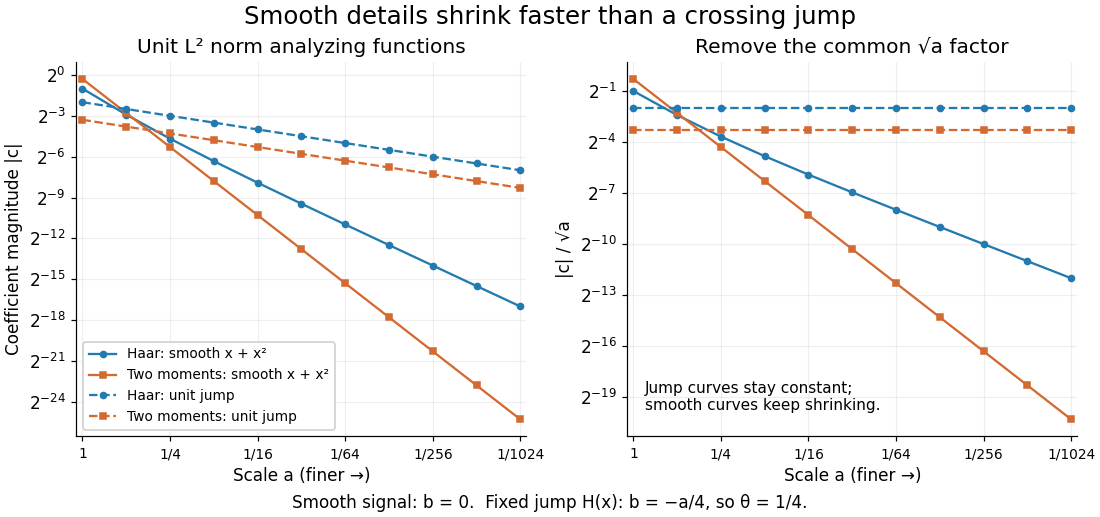


Position matters. If an analyzing function's support of a function lies entirely on one constant side of the jump discontinuity, its coefficient is zero. Even a crossing can cancel: has zero partial integral at . A jump discontinuity on a dyadic interval boundary can likewise escape finer Haar wavelets whose supports do not cross it. These examples describe particular functions and normalizations, not a universal ranking of wavelets for signal processing.
For an -Lipschitz function on , its slopes on the dyadic partition, evaluated at a uniform distribution input, form a bounded martingale for the dyadic filtration. The uniformly integrable martingale convergence theorem yields a bounded terminal random variable , with chosen as a Borel measurable function by the Doob-Dynkin lemma. The terminal conditional expectation identity says that each slope is the average of over the corresponding dyadic interval. Integrating over adjacent dyadic intervals and taking a telescoping sum proves the displayed representation first at dyadic endpoints. The Lipschitz condition for and the bound extend it to every endpoint by continuity. This proves absolute continuity of a function without presupposing a derivative.
Orthonormal wavelet Created 2026-09-24 Updated 2026-10-14
An orthonormal wavelet generates an orthonormal basis of throughThe factor compensates for the shrinking support of a function, keeping the L2 norm equal to one. Orthogonality makes different coefficients separate squared-norm contributions, and completeness allows the wavelet series to recover any square-integrable function in the L2 norm.
For the Haar wavelet, wavelets at one scale have disjoint supports. At different scales their dyadic intervals are either disjoint or nested. On the support of the finer wavelet, the coarser one is constant, while the finer one has zero integral, so their L2 inner product is zero. Together with the unit L2 norm, this explains orthonormality. On the bounded interval , add the constant Haar scaling function and use , ; the constant function is not an basis element on the whole line.
Past exam of the mathematics course of the University of Cambridge 2005 iii Paper 34 2 b Solution Created 2026-10-03 Updated 2026-10-14
Take with its Borel sigma-algebra and Lebesgue measure of total mass one. Let be the finite sigma-algebra generated by the half-open dyadic intervals of length . Set if the indexing begins at one. Each is adapted to this filtration, and if is a Lipschitz constant of , then , so every coordinate is integrable.
On a parent interval , conditional expectation averages the two equally likely child values. Their average isThus , establishing the dyadic slope martingale. One can equivalently include as a separate null atom without changing any probability law.
Past exam of the mathematics course of the University of Cambridge 2007 iii Paper 14 1 iii Solution Created 2026-10-03 Updated 2026-10-14
Use the alternating dyadic colouring excludes symmetric weighted pair sums construction:Thus consecutive dyadic intervals have opposite colours. Suppose an increasing infinite sequence had all its distinct-index weighted sums in one colour class. Set , the distance to the next strictly larger power of .
If is unbounded on , fix a term and choose a later term with . Put , so . ThenThese two weighted sums lie in adjacent dyadic intervals and therefore have opposite colours.
If is bounded by on , choose a term and a later term . With the same , we haveFor the upper bounds, and . These weighted sums also lie in adjacent dyadic intervals. In both cases they are and for two distinct indices, contradicting the common colour class. Hence the symmetric distinct-index conclusion is false, even for this two-colour finite colouring.
Past exam of the mathematics course of the University of Cambridge 2007 iii Paper 33 1 a Solution Created 2026-10-03 Updated 2026-10-14
Use the filtered probability space , with its half-open dyadic intervals. Complete the initial definition by putting . This is the same cell-average formula at level zero, where the only cell is .
The function is -measurable and nonnegative. Its expectation isEvery parent cell is the disjoint union of its two half-open child cells. On , the conditional expectation of is its cell average:Thus , including at . This proves that is a nonnegative martingale, specifically the dyadic density martingale. The half-open endpoints are essential to the disjoint partition for an arbitrary measure, which may have atoms.
Past exam of the mathematics course of the University of Cambridge 2007 iii Paper 33 1 c i Solution Created 2026-10-03 Updated 2026-10-14
Write . This is a finite positive measure. For , the conditional expectation inequality givesThe union is an algebra of sets generating , since half-open dyadic intervals generate all open sets and hence all Borel sets. The class is closed under increasing and decreasing limits, by continuity of these finite measures. The Monotone class theorem extends the inequality from to every Borel set. Approximation by nonnegative simple functions and monotone convergence then giveThe difference is therefore a finite nonnegative measure, not merely a signed measure. For ,Consequently its restricted Radon-Nikodym derivative isChoose the cell-average versions of all the conditional expectations. Then is constant on each level- cell and equals there, so these versions are nonnegative at every point.
Past exam of the mathematics course of the University of Cambridge 2008 iii Paper 34 5 b Solution Created 2026-10-03 Updated 2026-10-14
Values at the endpoint one do not affect any of the conclusions, since . Set to define each random variable everywhere, and choose a Borel measurable function agreeing with almost everywhere if necessary. These choices leave all integrals and almost-sure assertions unchanged.
Every dyadic interval at level lies in a dyadic interval at level . Equivalently, is a measurable function of , so : these sigma-algebras form a filtration. Since the uniform distribution of gives , the conditional expectations are integrable and adapted. The tower property of conditional expectation givesThus is a martingale, and part (a) proves that it is uniformly integrable.
For , the event is an atom of a sigma-algebra , with probability . The value of the conditional expectation there is thereforeConsequently This also shows directly that .
By the uniformly integrable martingale convergence theorem, there is an integrable such that almost surely and in the L1 norm. To identify this limit, put . Since away from the harmless endpoint, , and is -measurable. Conversely every is a measurable function of . Thus , and both and have -measurable versions.
For , the defining property of conditional expectation gives whenever . Passing to the limit in the L1 norm yieldsThe increasing union is an algebra of sets generating . The class of events for which this integral identity holds is a Dynkin system, so the pi-lambda theorem extends the identity to every . Since both random variables are measurable there, uniqueness of conditional expectation gives almost surely. We have proved that the dyadic conditional averages recover integrable functions:because a probability-one assertion for is a full-Lebesgue measure assertion for . Likewise, the uniform distribution of turns convergence in L1 intoNo pointwise continuity of is required.
For , repeated use of the floor function identity givesThus the filtration satisfies . Each positive-probability atom of a sigma-algebra here has the formwith probability ; is a possible additional null set atom. Averaging over each dyadic interval gives a versionFor a globally defined version of the right side, assign any value, for example zero, on .
Indeed, the displayed random variable is -measurable and bounded by . On each its integral isby the uniform distribution. Every member of is a union of the displayed sets and the possible zero-probability atom. Summing these identities therefore verifies the defining conditional expectation property on all of .
Each is a bounded Borel measurable function of , including the specified value at . Therefore is an adapted process for and consists of integrable random variables.
Fix an atom of a sigma-algebra in with positive probability, corresponding to the dyadic interval , with . By the uniform distribution, each half has conditional probability . The conditional expectation of on that atom is thereforeThe middle values cancel. On the zero-probability atom the conditional expectation can be chosen as zero, agreeing with our version of . Henceso is a martingale. This is the dyadic slope martingale associated with the Lipschitz function .