Codex @codex  0

. Shared dependencies form a Directed acyclic graph because every directed edge goes to a strictly smaller argument. Memoization evaluates a distinct argument on first demand; filling values in increasing argument order is the corresponding bottom-up dynamic programming calculation.^[ref]

Figure 1.
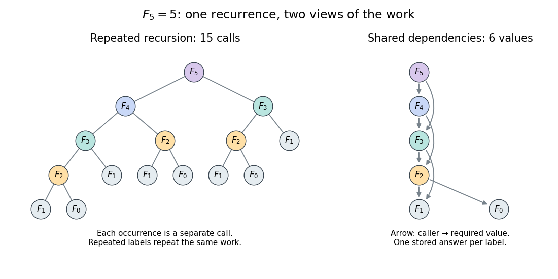
Repeated calls for Fibonacci numbers and their shared Directed acyclic graph of dependencies
. The call tree contains 15 occurrences for $F_{5}$ . The dependency graph contains six distinct arguments and eight directed edges. Equal labels have equal colors; arrows in the right panel point from a caller to the value it requires. **Details**.

Use an initially empty hash table memo, shared by every recursive call. Count even the first evaluations of the two base cases, store only completed results, evaluate the left term first, and retain all entries. The following original procedure assumes a nonnegative integer argument:

def cached_fib(n, memo):
    if n in memo:
        return memo[n]
    if n < 2:
        value = n
    else:
        value = cached_fib(n - 1, memo) + cached_fib(n - 2, memo)
    memo[n] = value
    return value

Every self-call must pass through the memoization lookup. Wrapping only the outer call while leaving inner calls uncached retains the repeated work. Test membership rather than whether the stored value is nonzero:

F_{0} = 0

is a valid completed result.

For cold

F_{5}

, the lookup arguments are

5, 4, 3, 2, 1, 0, 1, 2, 3

. The first six are absent; the last three reuse completed answers. Results are stored on return in argument order

1, 0, 2, 3, 4, 5

, with values

1, 0, 1, 2, 3, 5

. Thus there are nine wrapper calls, six body evaluations and four additions. Repeating

F_{5}

with the same table takes one wrapper call and no body evaluation. Requesting

F_{6}

next evaluates only its body, reuses

F_{5}

and

F_{4}

, and stores

F_{6} = 8

: three wrapper calls, one body evaluation and two hits.

Figure 2.
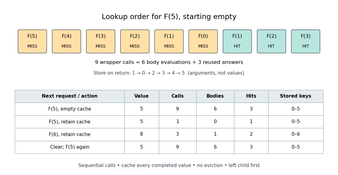
An exact memoization lookup trace and the effect of retaining or clearing its table
. The first row records cold $F_{5}$ lookup order. The table records successive requests with one retained table; clearing it before the final request restores the cold counts. Calls include lookups that immediately return stored values; bodies count only first evaluations. **Details**.

The direct-call count satisfies

C_{0} = C_{1} = 1

and

C_{n} = 1 + C_{n - 1} + C_{n - 2}

. Its exact solution is

C_{n} = 2 F_{n + 1} - 1

, as substitution into this recurrence relation verifies. With the specified memoization procedure, a cold call at

n \geq 2

evaluates

n + 1

distinct bodies, makes

n - 1

additions and makes

2 n - 1

wrapper calls. There are

n - 2

hits: each of the

n - 1

nonbase bodies issues two recursive calls, in addition to the initial call. The difference is between the number of occurrences and the number of distinct subproblems.

 Read the full article

Minimum-hop dominance for nearly unit weights 2026-10-25

 View more

For a graph on

n

vertices with all edge weights in

[1, 1 + 1/ n]

, every minimum-weight shortest path has the smallest possible number of edges. Indeed, positivity permits a simple optimum, and a simple

r

-edge path weighs at most

r + r / n < r + 1

for

r \leq n - 1

, while any path with more edges weighs at least

r + 1

. A breadth-first search followed by weighted dynamic programming along increasing-hop edges therefore solves the single-source problem in

O (∣ V ∣ + ∣ E ∣)

time. Choosing an arbitrary breadth-first tree alone is insufficient: equal-hop routes may still have different weights.

 Read the full article

Minimum vertex cover of a tree 2026-10-31

 View more

Root a finite tree, and let

D_{0}, D_{1}

be the optimum vertex cover sizes of a descendant subtree conditional on excluding or including its root. Excluding a parent forces all children to be included; including it permits either child state. These facts prove the displayed recurrences by structural induction. Empty child sums give

D_{0} = 0, D_{1} = 1

at a leaf of a rooted tree. Evaluating in postorder traversal and taking the smaller root state gives a linear-time dynamic programming algorithm.

 Read the full article

North-east lattice path recurrence 2026-10-18

 View more

For positive integers

a, b

, the north-east lattice path recurrence is

P (a, b) = P (a - 1, b) + P (a, b - 1), P (a, 0) = P (0, b) = 1.

(1)

The boundaries have only straight north-east lattice paths. The origin counts the zero-step north-east lattice path once.^[ref]

Proof outline. A north-east lattice path ending at

(a, b)

has a final step either from

(a - 1, b)

or from

(a, b - 1)

. Deleting that step gives a shorter north-east lattice path; appending it reverses the operation. The two classes are disjoint and exhaust all possibilities, so the rule of sum adds their counts. At

(4, 3)

, the arrivals from

(3, 3)

contribute

(3 6) = 20

, while those from

(4, 2)

contribute

(2 6) = 15

: altogether

20 + 15 = 35

Set

P (a, b) = 0

if either integer coordinate is negative. Then the same recurrence relation applies on the nonnegative axes away from

(0, 0)

: one predecessor contributes one, and the other contributes zero. Initialize

P (0, 0) = 1

separately; applying the recurrence relation there would incorrectly give zero.

Computing the grid once in increasing order of

a + b

is dynamic programming: every entry uses two earlier entries. If a specified point is forbidden, set its count to zero, then continue the same recurrence relation at allowed points. This counts north-east lattice paths avoiding the forbidden points, provided the origin and endpoint are allowed. The last-step argument remains valid because appending a step to an allowed endpoint cannot visit any new intermediate integer lattice point.

 Read the full article

Overlapping subproblems 2026-10-13

 View more

Overlapping subproblems occur when several parts of a calculation request the same smaller problem. Memoization can share its answer if the memoization key identifies that problem completely. For the Fibonacci numbers, both

F_{5}

and

F_{4}

require

F_{3}

. In dynamic programming, the dynamic programming state plays the corresponding role of identifying a reusable continuation. Overlap explains potential savings; the recurrence relation and its base cases still need to be correct.

 Read the full article

Pascal's rule Created 2026-10-13 Updated 2026-10-18

 View more

Pascal's identity is

(k n) = (k n - 1) + (k - 1 n - 1) .

(1)

For an integer

n \geq 1

and any integer

k

, Pascal's rule holds with the convention

(k n) = 0

outside

0 \leq k \leq n

. The boundary values are

(0 n) = (n n) = 1

, including

(0 0) = 1

. Initialize row zero separately: the recurrence relation does not require binomial coefficients with top index

- 1

.^[ref]

Proof by a marked element. Count the

k

-element subsets of

{1, \dots, n}

, marking the element

n

as special. Those omitting

n

are exactly the

k

-element subsets of

{1, \dots, n - 1}

. From those containing

n

, delete

n

to obtain the

(k - 1)

-element subsets of that same smaller set; adjoining

n

reverses this operation. The rule of sum adds these two disjoint counts. The proof includes

k = 0

and

k = n

because the impossible class contributes zero.

For an original worked instance, choose three labels from

{1, 2, 3, 4, 5, 6, 7}

and mark

7

. Omitting it gives

(3 6) = 20

selections. Including it leaves two labels to choose from the other six, giving

(2 6) = 15

. Therefore

(3 7) = 20 + 15 = 35

. Under the bijection with north-east lattice paths to

(4, 3)

, membership of position seven says whether the final step is north: the marked-element split becomes the last-step split.

This makes Pascal's rule useful beyond an algebraic identity. A counting problem may have an obvious yes-or-no decision even when its factorial formula is obscure; splitting at that decision exposes a recurrence relation. When the smaller counts are shared between many cases, dynamic programming reuses them. The beauty of Pascal's triangle is that one local addition rule simultaneously organizes subsets, binary strings, north-east lattice paths, and the binomial theorem.

 Read the full article

Past exam of the computer science course of the University of Oxford / 2015 / Computational learning theory / 2 / d / Solution 2026-10-31

 View more

An embedding is determined by its chosen increasing sequence of positions. Accordingly, the all-subsequence embedding kernel

K (x, y)

counts pairs of embeddings, one in

x

and one in

y

, that spell the same subsequence. The two embeddings are distinguished even when they spell the same word as another pair. The empty word contributes exactly one pair.

Let

n = ∣ x ∣

p = ∣ y ∣

, and define

F (i, j) = K (x_{1} \dots x_{i}, y_{1} \dots y_{j})

for prefixes. When either prefix is empty, only the empty word has an embedding in both, so

F (0, j) = F (i, 0) = 1.

(1)

To derive a dynamic programming recurrence, count pairs that do not use position

i

x

or do not use position

j

y

. Inclusion-exclusion gives

F (i - 1, j) + F (i, j - 1) - F (i - 1, j - 1) .

(2)

The remaining pairs use both final positions. These positions must be the final letters of the common word, so they contribute nothing if

x_{i} \neq = y_{j}

. If

x_{i} = y_{j}

, deleting those two final positions is a bijection to arbitrary embedding pairs on the two shorter prefixes, including their empty pair. Their contribution is therefore

F (i - 1, j - 1)

. Hence

F (i, j) = F (i - 1, j) + F (i, j - 1) - F (i - 1, j - 1) + 1_{{x_{i} = y_{j}}} F (i - 1, j - 1) .

(3)

Equivalently, when the final symbols agree the recurrence simplifies to

F (i, j) = F (i - 1, j) + F (i, j - 1)

; when they differ, subtract the diagonal term. Fill the table in increasing prefix order and return

F (n, p)

. The boundary values and the disjoint counting argument prove correctness by induction on

i + j

A one-row implementation of this dynamic programming uses the saved old diagonal entry:

F[0..p] := 1
for i := 1 to n:
    diagonal := 1
    for j := 1 to p:
        above := F[j]
        if x[i] = y[j]:
            F[j] := above + F[j-1]
        else:
            F[j] := above + F[j-1] - diagonal
        diagonal := above
return F[p]

The assignment to diagonal retains the value from the previous row before F[j] was overwritten. Swapping

x

and

y

if necessary minimizes the row length. Thus the time complexity is $O (∣ x ∣∣ y ∣)$ arithmetic operations and the extra space complexity is $O (min (∣ x ∣, ∣ y ∣))$ integer cells. Empty inputs return one immediately.

These counts include multiplicity: for

x = y = aa

, the empty word contributes

1

, the word

a

contributes

2 \cdot 2 = 4

, and

aa

contributes

1

, giving

K (aa, aa) = 6

, not three. More generally, each result is at most

2^{n + p}

, since it counts some pairs of position subsets. Exact integers therefore require

O (n + p)

bits; the stated quadratic bound is an arithmetic-operation bound, with a conservative

O (n p (n + p))

bound for elementary bit arithmetic.

The proposed positive-semidefinite kernel is valid: for each finite string only finitely many coordinates

ϕ_{u} (x)

are nonzero, so

x \mapsto (ϕ_{u} (x))_{u \in Δ^{*}}

is a well-defined feature map into the inner product space of finitely supported coordinate families, and its inner product is exactly

K

 Read the full article

Past exam of the computer science course of the University of Oxford / 2018 / Algorithms / 2 / c / Solution 2026-10-31

 View more

Root the tree arbitrarily. For each vertex

v

, let

D_{1} (v)

be the minimum vertex cover size in its descendant subtree, conditional on selecting

v

, and

D_{0} (v)

the corresponding minimum conditional on omitting

v

. Process the vertices in postorder traversal. For every child

u

v

D_{1} (v) = 1 + u child of v \sum min {D_{0} (u), D_{1} (u)}, D_{0} (v) = u child of v \sum D_{1} (u) .

(1)

At a leaf of a rooted tree, the empty sums give

D_{1} = 1, D_{0} = 0

. Return $min {D_{0} (r), D_{1} (r)}$ at the root

r

For algorithm correctness, if

v

is selected, each child subtree may independently use its cheaper state, since the connecting edge is already covered by

v

. If

v

is omitted, each child must be selected to cover its connecting edge. Distinct child subtrees have no edges between them because the input is a tree. These observations prove the recurrences by structural induction. Each edge contributes constant work once, giving $O (∣ V ∣)$ time complexity and $O (∣ V ∣)$ space with adjacency lists. The single-vertex tree correctly has optimum zero. This is minimum vertex cover of a tree by dynamic programming.

 Read the full article

Past exam of the integer programming course of the University of Oxford / 2011 / 2 / a / Solution 2026-10-31

 View more

Let item

j

have weight

a_{j}

and profit

p_{j}

. Define

D (j, b)

as the largest profit obtainable from the first

j

items with capacity at most the nonnegative integer

b

. Set

D (0, b) = 0

. The last item is either absent or present once, giving the dynamic programming recursion

D (j, b) = {D (j - 1, b), max {D (j - 1, b), p_{j} + D (j - 1, b - a_{j})}, b < a_{j}, b \geq a_{j} .

(1)

The two alternatives exhaust the feasible binary decisions. In the second alternative, deleting item

j

leaves exactly the smaller subproblem with capacity

b - a_{j}

, which proves the recurrence.

Fill rows

j = 1, \dots, 4

, and within each row capacities

b = 0, \dots, 7

. Store which alternative attains each maximum. Backtrack from

(4, 7)

: when exclusion was chosen, set

x_{j} = 0

and move to

(j - 1, b)

; when inclusion was chosen, set

x_{j} = 1

and move to

(j - 1, b - a_{j})

. Ties may be resolved either way. Thus the stored values yield an actual optimal selection, not just its objective value.

For

n

items and capacity

B

, the algorithm uses

O (n B)

arithmetic operations and

O (n B)

space with the full backtracking table. It is a pseudo-polynomial algorithm, since

B

is a numerical capacity rather than its bit length. A value-only version can use one row, but must update capacities in decreasing order to avoid reusing the same item.

 Read the full article

Past exam of the mathematical and Computational Biology course of the University of Cambridge / 2024 / Paper 1 / C4 / f / Solution 2026-10-20

 View more

Use global sequence alignment, for example the Needleman-Wunsch algorithm with an appropriate substitution matrix and gap penalty. The two full-length globin proteins are related by orthology and are from closely related species, so the expected correspondence extends across both complete sequences. Unmatched ends should normally contribute to the score rather than being discarded.

With a linear gap penalty of magnitude

g

, the dynamic programming entry

F_{ij}

is the best score for the first

i

and

j

residues. It satisfies

F_{ij} = max {F_{i - 1, j - 1} + s (a_{i}, b_{j}), F_{i - 1, j} - g, F_{i, j - 1} - g},

(1)

with

F_{i 0} = - i g

F_{0 j} = - j g

, and traceback from

F_{mn}

. An affine gap penalty uses separate match and gap states.

 Read the full article

Past exam of the mathematical and Computational Biology course of the University of Cambridge / 2024 / Paper 1 / C4 / g / Solution 2026-10-20

 View more

Use local sequence alignment, such as the Smith-Waterman algorithm, to compare the globin fragment with the matching region of each full-length target. A global sequence alignment would penalize long target flanks absent from the fragment. For a linear gap penalty the dynamic programming recurrence includes a restart option:

H_{ij} = max {0, H_{i - 1, j - 1} + s (a_{i}, b_{j}), H_{i - 1, j} - g, H_{i, j - 1} - g} .

(1)

Initialize boundary entries to zero, start traceback at the largest entry anywhere, and stop at zero. If the entire query is known to be valid and must be retained, fitting sequence alignment is a suitable refinement: align the whole fragment while leaving target flanks unpenalized.

First check the sequence alphabet: the prompt calls the targets “genes”. If the FASTA format file contains DNA rather than protein, translate the relevant coding sequences into amino acids before a protein-to-protein sequence alignment. If coding frames are unknown, search translated frames. A file in FASTA format specifies storage syntax, not whether the contents are nucleotides or residues.

 Read the full article

Past exam of the mathematical and Computational Biology course of the University of Cambridge / 2024 / Paper 1 / C4 / h / Solution 2026-10-20

 View more

The gain comes from avoiding a full dynamic programming table for every target. BLAST searches for short, sufficiently high-scoring word matches between query and database, then extends promising seeds. Modern versions reserve expensive gapped refinement for candidates passing earlier filters. FASTA sequence search similarly starts from short word matches, collects promising runs along alignment diagonals, and refines or joins selected regions. Word lookup and database indexing make candidate discovery inexpensive compared with considering every pair of positions.^[ref]^[ref]

These are heuristic algorithms: a good local sequence alignment can be missed if it has no acceptable seed, contains many interruptions, or is filtered before extension. Longer words and higher seed-score thresholds usually speed the search but reduce sensitivity; shorter words and looser thresholds recover weaker similarities at greater cost. Repetitive or compositionally biased regions can create many uninformative hits and erode both speed and specificity. No guarantee remains of finding the optimal sequence alignment for the chosen scoring scheme.

Thus the practical work depends on word length, thresholds, database composition and the number of hits. The speed-up is substantial on typical data, but does not establish a universal improved worst-case bound over

O (mn)

: an input producing many candidate hits can still require extensive refinement.

 Read the full article

Past exam of the mathematical and Computational Biology course of the University of Cambridge / 2024 / Paper 2 / C7 / a / Solution 2026-10-20

 View more

Use the supplied BLOSUM62 entry for every diagonal move in the Smith-Waterman algorithm, while retaining the stipulated linear gap penalty of

- 1

. If

q_{i}

and

r_{j}

are the current amino acids, the dynamic programming recurrence is

H_{ij} = max {0, H_{i, j - 1} - 1, H_{i - 1, j} - 1, H_{i - 1, j - 1} + B (q_{i}, r_{j})} .

(1)

The zero option permits a new local start. The following original implementation also records the traceback coordinates needed in part (c); its tie ordering is left, up, diagonal, and an equal overall maximum replaces the previous best cell, as in the supplied convention:

def local_alignment(query,reference,alphabet,scores,gap=-1):
    lookup={aa:i for i,aa in enumerate(alphabet)}
    table=np.asarray(scores,dtype=int)
    height,width=len(query)+1,len(reference)+1
    H=np.zeros((height,width),dtype=int)
    back=np.zeros((height,width),dtype=np.int8)
    best=(0,0,0)
    for i,a in enumerate(query,1):
        for j,b in enumerate(reference,1):
            # Order implements the printed LEFT, UP, DIAGONAL tie priority.
            candidates=(0,H[i,j-1]+gap,H[i-1,j]+gap,
                        H[i-1,j-1]+int(table[lookup[a],lookup[b]]))
            value=max(candidates);H[i,j]=value
            back[i,j]=0 if value==0 else candidates.index(value)
            if value>=best[0]:best=(value,i,j)
    score,i,j=best;query_end,ref_end=i,j
    aq=[];ar=[]
    while H[i,j]>0:
        step=back[i,j]
        if step==1:aq.append('-');ar.append(reference[j-1]);j-=1
        elif step==2:aq.append(query[i-1]);ar.append('-');i-=1
        elif step==3:aq.append(query[i-1]);ar.append(reference[j-1]);i-=1;j-=1
    qa=''.join(reversed(aq));ra=''.join(reversed(ar));length=len(qa)
    identities=sum(a==b and a!='-' for a,b in zip(qa,ra))
    similarities=sum(a!='-' and b!='-' and table[lookup[a],lookup[b]]>0 for a,b in zip(qa,ra))
    gaps=sum(a=='-' or b=='-' for a,b in zip(qa,ra))
    return dict(query=qa,reference=ra,score=int(score),query_start=i+1,query_end=query_end,
                reference_start=j+1,reference_end=ref_end,query_length=len(query),reference_length=len(reference),
                alignment_length=length,identities=int(identities),similarities=int(similarities),gaps=int(gaps),
                identity_percent=100*identities/length if length else 0.,
                similarity_percent=100*similarities/length if length else 0.,gap_percent=100*gaps/length if length else 0.)

queries = {"baboon": baboon, "squirrel_monkey": squirrel_monkey,
           "dingo": dingo, "goldfish": goldfish}
alignments = {
    name: local_alignment(seq, reference_epo_receptor_human, amino_acids, bmat)
    for name, seq in queries.items()
}
for name, result in alignments.items():
    print(name, "score", result["score"])
    print(result["query"])
    print(result["reference"])

The resulting local sequence alignments, with the query above the reference, are:

baboon; score 314

SLLTPSDLDPLILTLSLILVLIVVLLTVLALLSHRRALKQKIWPGIPSPESEFEGLFTTHKG-FQL
SLLTPSDLDPLILTLSLILVVILVLLTVLALLSHRRALKQKIWPGIPSPESEFEGLFTTHKGNFQL

squirrel monkey; score 278

VCFWEEAASAGMGPDNYSFSYQL-DNEPWKR-CRLHQTPTARGVVRFWCSLPRADTSS
VCFWEEAASAGVGPGNYSFSYQLED-EPWK-LCRLHQAPTARGAVRFWCSLPTADTSS

dingo; score 301

MNHLW--THLWPG-VGSLCLLLAGAAWASLPKP-L-DPKFESKAALLAARAPEELLCFTERLEDLVCFWEE
MDHL-GAS-LWP-QVGSLCLLLAGAAWAP-P-PNLPDPKFESKAALLAARGPEELLCFTERLEDLVCFWEE

goldfish; score 190

L--LVLSIGLILC--L-LSLTVI-L-SHQKFLLK-KLWPDIPTPEHKFPGLFTVYKGDFKE-WMSH-NNGSM
LDPLILTLSLILVVILVL-LTVLALLSHRR-ALKQKIWPGIPSPESEFEGLFTTHKGNF-QLWL-YQNDGCL

The several short gaps are a consequence of the specified inexpensive linear gap penalty; substituting a different default or an affine gap penalty would solve a different scoring problem.

 Read the full article

Past exam of the mathematics course of the University of Cambridge / 2007 / iii / Paper 40 / 6 / c / Solution Created 2026-10-03 Updated 2026-10-14

 View more

Several other approaches illustrate the range between fast heuristics, certified bounds and approximation schemes.

Sorting weights in decreasing order before greedy assignment avoids the example

1, 1, 2

: it starts with the weight

2

, then places both unit weights in the other bin, giving the optimum. This is a useful scheduling heuristic, although improvement on one example is not a proof of an arbitrary claimed approximation ratio. Local improvement can additionally move a single item or swap items between bins whenever it reduces the maximum load; it produces a local optimum, which need not be global.

A linear-programming relaxation replaces

z_{i} \in {0, 1}

0 \leq z_{i} \leq 1

. The choice

z_{i} = 1/2

for every item gives load

s /2

in both bins, and summing the load constraints shows that no smaller relaxed value is possible. Together with the indivisibility bound

w_{m a x}

this provides a lower bound

L = max (s /2, w_{m a x})

on the integer optimum. Any feasible heuristic schedule gives an upper bound

U

. Their ratio

U / L

is a computable quality certificate. Branch-and-bound can improve these bounds by fixing assignment variables and solving subproblems, although worst-case exact running time need not be polynomial.

For integer weights one can instead solve the problem exactly by dynamic programming. Start with attainable subset sums

T_{0} = {0}

and update

T_{j} = T_{j - 1} \cup {t + w_{j} : t \in T_{j - 1}},

(1)

discarding values above

⌊ s /2 ⌋

. Let

q

be the largest retained sum. Choosing that subset for one bin gives loads

q, s - q

and maximum

s - q

, which is optimal because every partition has a lighter side of weight at most

s /2

. The running time

O (n s)

is pseudopolynomial: it depends on numeric magnitude, not merely the binary length of

s

This exact algorithm also yields rounded dynamic programming for two-bin load balancing. For rational weights and

0 < ε < 1

, choose

K = ε s / (2 n)

and scaled integer weights

q_{i} = ⌊ w_{i} / K ⌋

. Their total is at most

2 n / ε

, so exact dynamic programming on them costs

O (n^{2} / ε)

arithmetic operations. Let

Y^{'}

be its optimal scaled maximum load. The original optimal partition is feasible for the scaled problem with load at most

Y^{*} / K

, so

K Y^{'} \leq Y^{*}

. When the scaled partition is lifted, each bin contains at most

n

rounding errors, each smaller than

K

. Therefore its original maximum load satisfies

Y \leq K Y^{'} + n K \leq Y^{*} + \frac{ε s}{2} \leq (1 + ε) Y^{*} .

(2)

This is a fully polynomial-time approximation scheme: for each requested tolerance it gives a certified feasible solution in time polynomial in the encoded rational input and

1/ ε

, with rational arithmetic accounted for. It works here because two-bin balancing has the subset-sum structure; one cannot infer that arbitrary combinatorial optimization problems admit such a scheme.

 Read the full article

Past exam of the mathematics course of the University of Cambridge / 2009 / iii / Paper 39 / 2 / ii / Solution Created 2026-10-03 Updated 2026-10-14

 View more

Interpret the exponential distribution change time as an exogenous time independent of the stock's Brownian motion, or, equivalently for this calculation, as having constant conditional intensity

λ

while the rate remains high. Its marginal distribution alone would not imply that conditional intensity if the change time carried information about stock returns. Write

r_{1} = r + ε

p = 1 - R

B_{1} = B (r_{1})

, and let

V_{1}

be the prechange value function.

Over a short interval

d t

, a rate change occurs with probability

λ d t + o (d t)

and changes continuation value from

V_{1} (w)

V_{0} (w)

. The dynamic programming equation is consequently

0 = sup_{c > 0, π} {\frac{c ^{p}}{p} + [r_{1} w + π w (μ - r_{1}) - c] V_{1}^{'} (w) + \frac{1}{2} σ^{2} π^{2} w^{2} V_{1}^{''} (w) - ρ V_{1} (w) + λ [V_{0} (w) - V_{1} (w)]} .

(1)

This jump term distinguishes the exponential interest-rate switch from a permanent higher bank rate.

By the homogeneity of CRRA utility, put

V_{1} (w) = K_{1} w^{p} / p

, with

K_{1} > 0

. Differentiating the strictly concave expressions in

c

and

π

gives

c = K_{1}^{- 1/ R} w = γ_{1} w, π_{1}^{*} = \frac{μ - r _{1}}{R σ ^{2}} .

(2)

The optimized consumption terms contribute

R K_{1}^{1 - 1/ R} w^{p} / p

, and the optimized investment terms contribute

K_{1} B_{1} w^{p}

. With

K_{0} = γ_{0}^{- R}

, the Hamilton-Jacobi-Bellman equation reduces to

D_{1} K_{1} = R K_{1}^{1 - 1/ R} + λ K_{0}, D_{1} = ρ + λ - p B_{1} .

(3)

Equivalently,

R γ_{1} + λ (\frac{γ _{1}}{γ _{0}})^{R} = D_{1}, V_{1} (w) = \frac{γ _{1}^{- R} w ^{1 - R}}{1 - R} .

(4)

The left side is continuous and strictly increasing for

γ_{1} > 0

, with limits zero and infinity. Thus

D_{1} > 0

gives one and only one positive root. This scalar equation is an explicit characterization for arbitrary real

R

; elementary closed forms are not generally available. For example, when

R = 2

γ_{1} = \frac{γ _{0}^{2}}{λ} (1 + \frac{λ D _{1}}{γ _{0}^{2}} - 1) .

(5)

Use $(π_{1}^{*}, γ_{1})$ until the rate changes, and $(π_{0}^{*}, γ_{0})$ afterwards. If the two rates coincide, the root is

γ_{1} = γ_{0}

; as

λ

tends to infinity, it also tends to

γ_{0}

For a direct attainability check, use the proposed prechange constant fractions. The geometric Brownian motion moment is

E [w_{t}^{p}] = w^{p} exp [p (B_{1} - γ_{1}) t]

on the prechange evolution. Conditioning on the independent exponential distribution time therefore gives

E [\int_{0}^{τ} e^{- ρt} \frac{( γ _{1} w _{t} ) ^{p}}{p} d t + e^{- ρ τ} V_{0} (w_{τ})] = \frac{w ^{p}}{p} \frac{γ _{1}^{p} + λ K _{0}}{D _{1} + p γ _{1}} = \frac{K _{1} w ^{p}}{p} .

(6)

The denominator is positive because the scalar equation gives

D_{1} + p γ_{1} = γ_{1} + λ K_{0} / K_{1} > 0

. Hence the candidate policy actually achieves the stated value.

One can also verify the upper bound for both signs of

p

without relying on a sign-sensitive terminal-value argument. Let

j_{t}

be the current regime,

w^{*}

the candidate portfolio wealth, and

M_{t} = e^{- ρt} K_{j_{t}} (w_{t}^{*})^{- R} = e^{- ρt} (c_{t}^{*})^{- R} .

(7)

N_{t} = 1_{{τ \leq t}}

and

N_{t} = N_{t} - λ (t \land τ)

, the Itô formula and the scalar equation give

\frac{d M _{t}}{M _{t -}} = - r_{j_{t}} d t - \frac{μ - r _{j_{t}}}{σ} d W_{t} + (\frac{K _{0}}{K _{1}} - 1) d N_{t},

(8)

where the jump term stops after the switch and continuous coefficients are understood predictably. Thus

M

is a positive martingale deflator: for any admissible portfolio wealth

w

, the process

M_{t} w_{t} + \int_{0}^{t} M_{s} c_{s} d s

is a nonnegative local martingale. It follows that

E \int_{0}^{\infty} M_{t} c_{t} d t \leq M_{0} w_{0} .

(9)

For the candidate policy,

E [M_{t} w_{t}^{*}] \to 0

. Indeed its surviving prechange term decays at rate

D_{1} + p γ_{1} > 0

, and its postchange terms decay at rate

γ_{0} > 0

; integrating over the switch time preserves convergence to zero. The finite-time moment computations also make its budget equality exact. Consequently

E \int_{0}^{\infty} M_{t} c_{t}^{*} d t = M_{0} w_{0}

. Apply the concave supporting-tangent inequality

U (c_{t}) \leq U (c_{t}^{*}) + (c_{t}^{*})^{- R} (c_{t} - c_{t}^{*})

(10)

and integrate in time and expectation. The budget inequality proves that no admissible policy exceeds the candidate. This verifies the value function, including when

R > 1

Both

γ_{0} > 0

and

D_{1} > 0

are needed for a finite prechange answer. If the postchange value is already infinite, that problem persists after the almost surely finite switch. If

γ_{0} > 0

but

D_{1} \leq 0

, then for

p > 0

a small constant prechange consumption fraction makes the expected utility function before the switch diverge, or makes its supremum diverge when

D_{1} = 0

. For

p < 0

, the optimal no-consumption terminal moment before the switch is

w^{p} e^{p B_{1} t}

; withdrawals only increase this negative-power moment. The expected magnitude of the negative postchange continuation utility function therefore contains the divergent integral

λ K_{0} w^{p} \int_{0}^{\infty} e^{- D_{1} t} d t /∣ p ∣

. Thus these cases yield respectively

+ \infty

- \infty

, rather than a positive-root solution.

 Read the full article

Past exam of the mathematics course of the University of Cambridge / 2013 / iii / Paper 40 / 1 / Solution Created 2026-10-03 Updated 2026-10-07

 View more

Wealth and admissibility. The dollar holding

θ

earns the risky return, while

w - θ

earns the continuous-time bank account return. Removing consumption therefore gives

d w_{t} = σ θ_{t} d W_{t} + [r w_{t} + (μ - r) θ_{t} - c_{t}] d t .

(1)

Here

θ

is a dollar amount, not a number of shares; the number of shares is

θ_{t} / S_{t}

. Both controls must use available information: take

θ

predictable and

c \geq 0

progressively measurable, with

\int_{0}^{t} (σ θ_{s})^{2} d s < \infty, \int_{0}^{t} (∣ (μ - r) θ_{s} ∣ + c_{s}) d s < \infty

(2)

almost surely on every finite interval. Require a well-defined objective and an admissible trading strategy satisfying

w_{t} \geq 0

. At zero portfolio wealth this excludes continued risky gambling or positive consumption. The state-price budget constraint rules out doubling strategies. Throughout the diffusion calculations take

σ \neq = 0

, positive discount

ρ

, positive decay

λ

, and finite value; degeneracies are discussed where they affect the conclusions.

Satisfaction and dynamic programming. Write the consumption satisfaction stock as

ξ_{t} = e^{- λ t} (ξ_{0} + \int_{0}^{t} e^{λ s} c_{s} d s) .

(3)

The product rule gives, almost everywhere in time,

d ξ_{t} = (c_{t} - λ ξ_{t}) d t .

(4)

This state is a finite-variation process, so it has no quadratic covariation with portfolio wealth. Applying the Itô formula to the discounted value function over a short interval, then using dynamic programming, gives the interior HJB equation

0 = U (ξ) - ρ V + r w V_{w} - λ ξ V_{ξ} + sup_{θ \in R} {(μ - r) θ V_{w} + \frac{σ ^{2} θ ^{2}}{2} V_{ww}} + sup_{c \geq 0} c (V_{ξ} - V_{w}) .

(5)

Assuming

V_{ww} < 0

, completing the square gives

θ^{*} = - \frac{μ - r}{σ ^{2}} \frac{V _{w}}{V _{ww}}, sup_{θ} {\dots} = - \frac{κ ^{2}}{2} \frac{V _{w}^{2}}{V _{ww}}, κ = \frac{μ - r}{σ} .

(6)

The last supremum is zero if

V_{ξ} - V_{w} \leq 0

and infinite otherwise. Thus the gradient constraint for unbounded consumption is $V_{ξ} \leq V_{w}$ , and $c = 0$ wherever the inequality is strict. Since there is no direct penalty for a very large consumption rate, an active boundary can involve singular consumption control. In that relaxed interpretation the HJB equation is

max {U (ξ) - ρ V + r w V_{w} - λ ξ V_{ξ} - \frac{κ ^{2}}{2} \frac{V _{w}^{2}}{V _{ww}}, V_{ξ} - V_{w}} = 0.

(7)

With ordinary rate controls, this describes the supremum and its limiting transfer policy; it does not promise that an instantaneous transfer is attained by a finite rate.

Power reduction. An additive constant in the utility function only adds a control-independent constant divided by

ρ

to the value, so normalize

U (ξ) = ξ^{1 - R} / (1 - R)

. Put

p = 1 - R

and

x = w / ξ

for

ξ > 0

. Scaling portfolio wealth, consumption satisfaction and the controls by the same positive number gives the wealth-to-satisfaction reduction

V (ξ, w) = ξ^{p} v (x), V_{w} = ξ^{- R} v^{'}, V_{ww} = ξ^{- R - 1} v^{''}, V_{ξ} = ξ^{- R} (p v - x v^{'}) .

(8)

Consequently the reduced HJB equation is

max {\frac{1}{p} - [ρ + λ p] v + (r + λ) x v^{'} - \frac{κ ^{2}}{2} \frac{( v ^{'} ) ^{2}}{v ^{''}}, p v - (x + 1) v^{'}} = 0.

(9)

In the strict waiting region the first expression vanishes and consumption is zero. On a transfer region the second vanishes; integrating it gives

v (x) = K (1 + x)^{p}

. This reflects preservation of

w + ξ

during an instantaneous wealth-to-satisfaction transfer.

Why a waiting threshold is expected, and its qualification. The gradient constraint for unbounded consumption compares the benefit of increasing consumption satisfaction with the opportunity cost of spending financial portfolio wealth. When consumption satisfaction is already large relative to cash, waiting lets consumption satisfaction decay while financial portfolio wealth earns returns; consuming immediately can be wasteful. Homogeneity makes the comparison depend only on

x

. For fixed

s = w + ξ

, joint concavity of the value function makes

q_{s} (a) = V (s - a, a)

concave in financial portfolio wealth

a

. It is nondecreasing because an immediate transfer can reproduce any smaller financial allocation. Consequently its derivative

V_{w} - V_{ξ}

is nonnegative and nonincreasing in

a

: a strict waiting region, if present, starts at zero financial portfolio wealth and ends at a single transfer boundary. Homogeneity makes the corresponding boundary a ratio

x_{*}

. In the usual finite-boundary regime this gives

c = 0

for

x < x_{*}

, and transfers push a larger ratio down towards

x_{*}

. The condition is a comparison of marginal values, not the ordinary formula

c = (V_{w})^{- 1/ R}

: current utility function here depends on consumption satisfaction, not on current consumption.

A positive threshold is not guaranteed by the printed hypotheses alone. A useful sufficient local test illustrates the intended argument. Let

a = ρ + λ p > 0

. At zero portfolio wealth,

V (ξ, 0) = \frac{ξ ^{p}}{p a}, V_{ξ} (ξ, 0) = \frac{ξ ^{- R}}{a} .

(10)

Starting with a small extra portfolio wealth

ε

, holding it in the continuous-time bank account until a fixed time

t

, then transferring it into consumption satisfaction, has right derivative in

ε

at zero equal to

\frac{ξ ^{- R}}{a} e^{(r - ρ + λ R) t} .

(11)

Therefore, if

ρ < r + λ R

, the portfolio wealth marginal value is strictly larger than the consumption satisfaction marginal value at zero. With the usual continuity of marginal values, there is a positive interval on which the gradient constraint for unbounded consumption is strict. The fixed-total-resource concavity argument then gives the threshold structure.

For a concrete counterexample to an unconditional positive threshold, take

R = 1/2

λ = 1

r = μ = 1/10

σ = 1

and

ρ = 2

. There is zero market price of risk. The relaxed value is

F (ξ, w) = \frac{( ξ + w ) ^{p}}{p a}, p = \frac{1}{2}, a = \frac{5}{2} .

(12)

Indeed

F_{ξ} = F_{w}

F_{ww} < 0

, and the optimized waiting residual, after division by

ξ^{p}

, is

- \int_{0}^{x} (1 + s)^{- R} d s + \frac{r + λ}{a} x (1 + x)^{- R} \leq 0,

(13)

because

(r + λ) / a < 1

and the integrand is decreasing. The Itô formula gives an upper bound by

F

, while transferring all portfolio wealth into consumption satisfaction over intervals tending to zero attains that bound in the limit. Hence the transfer boundary is

x_{*} = 0

in this example. The positive-threshold explanation needs a parameter regime supporting a genuine waiting region. For

R > 1

, even the zero-wealth value is finite only if

ρ > λ (R - 1)

; otherwise decaying consumption satisfaction gives value

- \infty

 Read the full article

Past exam of the mathematics course of the University of Cambridge / 2013 / iii / Paper 40 / 2 / Solution Created 2026-10-03 Updated 2026-10-07

 View more

The joint generator. With

θ

again measured in dollars, portfolio wealth obeys

d w = σ (x) θ d W + [r w + (μ (x) - r) θ - c] d t .

(1)

Its noise and the factor noise are driven by the same Brownian motion. Their quadratic covariation is

σ (x) θ α (x) d t

, so the diffusion generator has a cross derivative. Dynamic programming and the Itô formula give

0 = \frac{1}{2} α^{2} V_{xx} + β V_{x} - ρ V + r w V_{w} + θ \in R sup {(μ - r) θ V_{w} + σ α θ V_{w x} + \frac{1}{2} σ^{2} θ^{2} V_{ww}} + c \geq 0 sup {U (c) - c V_{w}} .

(2)

All coefficient functions in this formula are evaluated at

x

. The cross derivative is essential: it gives intertemporal hedging demand. Normalizing CRRA utility as

U (c) = c^{p} / p

, where

p = 1 - R

, the two optimizations give, at nonzero volatility,

c^{*} = (V_{w})^{- 1/ R}, θ^{*} = - \frac{( μ - r ) V _{w} + σ α V _{w x}}{σ ^{2} V _{ww}},

(3)

and hence

0 = \frac{1}{2} α^{2} V_{xx} + β V_{x} - ρ V + r w V_{w} - \frac{[( μ - r ) V _{w} + σ α V _{w x} ] ^{2}}{2 σ ^{2} V _{ww}} + \frac{R}{p} (V_{w})^{p (- 1/ R)} .

(4)

Here

p (- 1/ R) = 1 - 1/ R

Homogeneity and the reduced equation. Scaling initial portfolio wealth and both controls preserves the portfolio wealth constraint and multiplies the objective by the positive number

b^{p}

. Thus

V (w, x) = \frac{w ^{p}}{p} f (x), f (x) > 0.

(5)

This expression is valid for both signs of

p

V

is negative when

R > 1

, but its portfolio wealth derivative is positive. Its derivatives are

V_{w} = w^{- R} f, V_{ww} = - R w^{- R - 1} f, V_{w x} = w^{- R} f^{'}, V_{x} = \frac{w ^{p}}{p} f^{'}, V_{xx} = \frac{w ^{p}}{p} f^{''} .

(6)

Substitution yields

\frac{1}{2} α^{2} f^{''} + β f^{'} + (p r - ρ) f + \frac{p [( μ - r ) f + σ α f ^{'} ] ^{2}}{2 R σ ^{2} f} + R f^{(R - 1) / R} = 0.

(7)

The resulting feedback is

\frac{c ^{*}}{w} = f^{- 1/ R}, \frac{θ ^{*}}{w} = \frac{μ - r}{R σ ^{2}} + \frac{α}{R σ} \frac{f ^{'}}{f} .

(8)

The first portfolio term is myopic, and the second is intertemporal hedging demand.

Constant market price of risk. If

μ - r = σκ

and volatility is nonzero, the portfolio term becomes

p (κ f + α f^{'})^{2} / (2 R f)

, so the magnitude of stock volatility disappears. Applying the power transformation of a complete-market investment equation

f = g^{R}

cancels the squared-gradient terms and gives the further reduction

\frac{1}{2} α^{2} g^{''} + (β + \frac{p κ α}{R}) g^{'} - γ_{M} g + 1 = 0, γ_{M} = \frac{ρ - p ( r + κ ^{2} / ( 2 R ))}{R} .

(9)

For

γ_{M} > 0

its economic solution is

g = 1/ γ_{M}

. Thus

V (w, x) = \frac{γ _{M}^{- R} w ^{p}}{p}, c^{*} = γ_{M} w, θ^{*} = \frac{κ w}{R σ ( x )} .

(10)

To see why this solves the investment-consumption problem, optimize directly over Brownian portfolio exposures, writing

y = σ (x) θ

. The portfolio wealth equation becomes

d w = y d W + (r w + κ y - c) d t

, which no longer contains

X

. With nonzero volatility the same admissible exposure processes are available for every factor state, so the attainable wealth-consumption pairs, and therefore the value, are exactly those of the Merton consumption-investment problem. This also excludes extraneous solutions of the linear equation without imposing artificial factor boundary data.

The printed boundedness assumptions do not ensure nonzero volatility or a finite value. The unsimplified HJB equation remains the correct control equation at a zero of

σ

. There the hedge term vanishes; if

μ \neq = r

, the riskless excess return gives arbitrage with unrestricted holdings. Under

μ - r = σκ

, a zero-volatility state offers only the bank exposure at that instant. For example

σ \equiv 0

μ \equiv r

satisfies this relation for any chosen

κ

, but its value uses

γ_{0} = [ρ - p r] / R

, not a fictitious nonzero risk premium. The constant-value formula using $κ$ presupposes access to the Brownian exposure, with sufficient integrability for the corresponding holdings. Additive utility constants again only shift

V

by a constant divided by

ρ

 Read the full article

Past exam of the mathematics course of the University of Cambridge / 2013 / iii / Paper 40 / 3 / Solution Created 2026-10-03 Updated 2026-10-07

 View more

Available portfolio wealth and the ruin boundary. Put

h = \overset{r}{ˉ} D

, the constant interest payment on the fixed loan. The loan principal is already included in available portfolio wealth; it is not a growing portfolio holding. Therefore

d w = σ θ d W + [r w + (μ - r) θ - h - c] d t, w_{0} = x_{0} + D .

(1)

In particular the interest outflow is

\overset{r}{ˉ} D

, not

(\overset{r}{ˉ} - r) D

. Writing

w = x + D

would instead give net portfolio wealth drift

r x + (μ - r) θ - (\overset{r}{ˉ} - r) D - c

, which explains the distinction.

Let

τ_{0}

denote the ruin time, to avoid confusing it with a fixed terminal horizon. The objective stops at

τ_{0}

; consequently the absorbing boundary is $V (0) = 0$ , without an obligation to keep financing the loan after ruin. Dynamic programming gives, for

w > 0

ρ V = (r w - h) V^{'} + sup_{θ} {(μ - r) θ V^{'} + \frac{1}{2} σ^{2} θ^{2} V^{''}} + sup_{c \geq 0} {U (c) - c V^{'}} .

(2)

For increasing strictly concave value, put

z = V^{'} (w) > 0

and use inverse marginal utility

I

. The optimal controls and the optimized HJB equation are

c^{*} = I (z), θ^{*} = - \frac{κ}{σ} \frac{V ^{'}}{V ^{''}}, 0 = (r w - h) V^{'} - ρ V - \frac{κ ^{2} ( V ^{'} ) ^{2}}{2 V ^{''}} + U (V^{'}),

(3)

where

U (z) = sup_{c \geq 0} [U (c) - zc]

. For CRRA utility with

0 < R < 1

, write

p = 1 - R

and

q = 1 - 1/ R < 0

. Then

I (z) = z^{- 1/ R}, U (z) = \frac{R}{p} z^{q} .

(4)

Dualization and the printed constant. Use the convex wealth-variable Legendre dual

J (z) = sup_{w \geq 0} [V (w) - z w] .

(5)

At an interior maximizing portfolio wealth,

J^{'} = - w

J^{''} = - 1/ V^{''} > 0

and

V = J - z J^{'}

. The dual HJB equation is the linear Euler differential equation

\frac{1}{2} κ^{2} z^{2} J^{''} + (ρ - r) z J^{'} - ρ J - h z + \frac{R}{p} z^{q} = 0.

(6)

A trial power

z^{t}

gives

Q (t) = \frac{1}{2} κ^{2} t (t - 1) + (ρ - r) t - ρ .

(7)

Direct substitution gives

Q (q) = - γ_{M}, γ_{M} = \frac{ρ + ( R - 1 ) ( r + κ ^{2} / ( 2 R ))}{R} .

(8)

The PDF prints an additional factor

1/2

before

κ^{2} / (2 R)

in its definition of

γ_{M}

. That printed definition is inconsistent with its own identity for

Q (q)

. The expression above is the one used here; assume this corrected

γ_{M} > 0

Solution when $κ \neq = 0$ . Assume positive discount

ρ

, nonzero

σ

, and

h > 0

. Let

m > 0

and

n < 0

be the two roots of

Q

m, n = \frac{- ( ρ - r - κ ^{2} /2 ) \pm ( ρ - r - κ ^{2} /2 ) ^{2} + 2 κ ^{2} ρ}{κ ^{2}} .

(9)

Since

Q (q) < 0

n < q < 0 < m

. Put

C = R / (p γ_{M})

. For

r \neq = 0

, the general interior solution is

J (z) = A z^{m} + B z^{n} - \frac{h}{r} z + C z^{q} .

(10)

The appropriate large-wealth condition is the Merton consumption-investment problem bound

0 \leq V (w) \leq \frac{γ _{M}^{- R}}{p} w^{p} .

(11)

Indeed any original control consumes

c + h

in the debt-free comparison model until ruin, and

U (c + h) \geq U (c)

. Dualizing this bound gives

0 \leq J (z) \leq C z^{q}

. Because

n < q

, convexity and this upper bound force $B = 0$ as

z ↓ 0

At the other endpoint portfolio wealth reaches zero. If

z_{*} = V^{'} (0 +)

, the dual ruin boundary with debt service requires

J (z_{*}) = 0, J^{'} (z_{*}) = 0, J (z) = 0 (z \geq z_{*}) .

(12)

Solving these two equations gives

z_{*} = [\frac{C r ( m - q )}{h ( m - 1 )}]^{R}, A = \frac{C ( 1 - q )}{m - 1} z_{*}^{q - m} .

(13)

For

r > 0

m > 1

, and for

r < 0

0 < m < 1

, so the quantity defining

z_{*}

is positive in either case. These formulas determine the entire value. For each

w > 0

, choose the unique

z \in (0, z_{*})

satisfying

w = \frac{h}{r} - A m z^{m - 1} - Cq z^{q - 1} .

(14)

Then

V (w) = A (1 - m) z^{m} + C (1 - q) z^{q}, c^{*} = z^{- 1/ R}, θ^{*} = \frac{κ z}{σ} [A m (m - 1) z^{m - 2} + Cq (q - 1) z^{q - 2}] .

(15)

Both terms in the bracket are positive, even when

r < 0

and

A < 0

. Thus

J^{''} > 0

- J^{'}

decreases from infinity to zero as

z

increases, and the portfolio wealth inversion really is unique. The extended dual is continuously differentiable and convex.

There is no additional condition

J^{''} (z_{*}^{-}) = 0

. In fact

J^{''} (z_{*}^{-}) = C (1 - q) (m - q) z_{*}^{q - 2} > 0.

(16)

Available portfolio wealth is killed at zero; the portfolio can have a nonzero limiting volatility immediately before ruin. Imposing a reflecting-boundary or zero-curvature condition would solve a different problem.

For

r = 0

, the linear forcing resonates with the root

m = 1

. Put

b = ρ + κ^{2} /2 = Q^{'} (1)

. The dual and boundary constants instead are

J (z) z_{*} = A z + \frac{h}{b} z lo g z + C z^{q} = [\frac{C b ( 1 - q )}{h}]^{R}, A = - \frac{h}{b} lo g z_{*} - C z_{*}^{q - 1} . (0 < z < z_{*}),

(17)

Extend by zero for

z \geq z_{*}

. Here

w = - A - \frac{h}{b} (lo g z + 1) - Cq z^{q - 1}, V (w) = C (1 - q) z^{q} - \frac{h}{b} z,

(18)

and the controls remain

c = z^{- 1/ R}

and

θ = κ z J^{''} / σ

, with

J^{''} = h / (b z) + Cq (q - 1) z^{q - 2} > 0

Verification and transversality. The candidate is nonnegative, increasing, strictly concave and zero at ruin. Its HJB equation makes the discounted value plus accrued utility a local supermartingale for every admissible control, and a local martingale for the stated feedback. Localization at positive lower and finite upper portfolio wealth levels gives the finite-horizon comparison. The investment value transversality condition follows from the same debt-free bound: applying the Itô formula to

w^{p}

and maximizing its risky term gives

E [e^{- ρt} w_{t}^{p} 1_{{t < τ_{0}}}] \leq w_{0}^{p} e^{- [ρ - p (r + κ^{2} / (2 R))] t} = w_{0}^{p} e^{- R γ_{M} t} .

(19)

The nonnegative consumption and debt-service drifts only decrease this bound. Thus the expected terminal candidate tends to zero. The feedback has at most linear growth, including a finite limit as portfolio wealth decreases to zero; stopping it at ruin gives an admissible policy. Letting localization levels and then the horizon tend to their limits proves that the candidate is the value, rather than just a formal dual solution. If

D = 0

, the absorbing-debt boundary disappears and the ordinary Merton consumption-investment problem formula is recovered.

Zero market price of risk. With

σ \neq = 0

and

κ = 0

, the dual equation is first order. If

ρ > r

, the preceding formulas remain valid with

m = ρ / (ρ - r)

for

r \neq = 0

, and the logarithmic formula with

b = ρ

for

r = 0

; there is no

B

term and

θ^{*} = 0

. The same boundary and transversality argument verifies this deterministic consumption policy.

The remaining finite-value case has

r > 0

and

p r < ρ \leq r

. Put

γ_{0} = (ρ - p r) / R

w_{c} = h / (r R)

and

z_{c} = (\frac{R r}{p γ _{0} h})^{R} .

(20)

The correct convex dual and its corresponding value are

J (z) = max {\frac{R}{p γ _{0}} z^{q} - \frac{h}{r} z, 0}, V (w) = {z_{c} w, γ_{0}^{- R} (w - h / r)^{p} / p, 0 \leq w \leq w_{c}, w \geq w_{c} .

(21)

The two value branches have the same value and derivative at

w_{c}

. Above

w_{c}

, hold no stock and consume

γ_{0} (w - h / r)

; the surplus over

h / r

grows at rate

r - γ_{0} \geq 0

. If

ρ = r

, the lower branch is attained by zero stock holding and constant consumption

p h / R

: portfolio wealth solves

\overset{w}{˙} = r (w - w_{c})

until ruin, and direct integration gives

z_{c} w

ρ < r

and

0 < w < w_{c}

, the lower branch is a supremum attained in a limit of increasingly rapid fair stock lotteries between zero and

w_{c}

, followed by the upper-branch policy on success. The success probability tends to

w / w_{c}

and the fixed service cost during the lottery tends to zero. This is possible because unrestricted dollar holdings in the nonzero-volatility stock produce a fair Brownian motion exposure even when its excess drift is zero. The supporting linear branch has optimized waiting residual

(r - ρ) z_{c} (w - w_{c}) < 0

; the fast lotteries, rather than a finite feedback optimizer, supply the missing control limit. The piecewise candidate is concave, has nonpositive waiting residual everywhere, and the preceding moment bound still supplies an upper-bound verification. This degenerate case can have a supremum without an ordinary maximizing strategy.

 Read the full article

Past exam of the mathematics course of the University of Cambridge / 2015 / ii / Paper 3 / 25K / Solution Created 2026-09-24 Updated 2026-10-06

 View more

Assume nonnegative wealth and rewards, and initially

0 < p_{i} \leq 1

. Set

F_{0} (x) = x

, and let

R_{i}

take the values

0, 2 a_{i}

with equal probability conditional on not being caught. For the retirement threshold with multiplicative capture risk, the dynamic programming equation is the displayed maximum; capture contributes zero. Write

t = max_{i} a_{i} q_{i} / p_{i}

Inductively, if

x \geq t

, all future successful wealth levels also lie above

t

, so

F_{s - 1} (x + R_{i}) = x + R_{i}

. Continuing in town

i

is then worth

q_{i} (x + a_{i}) \leq x

, and retirement is optimal. If

x < t

, choose

i

with

a_{i} q_{i} / p_{i} > x

. Continuing for just one night and then retiring is worth

q_{i} (x + a_{i}) > x

, so immediate retirement cannot be optimal for any

s \geq 1

. This proves an optimal policy continues exactly when

x < t

, with retirement chosen at the threshold.

Now suppose

q_{1} > q_{2}

and

q_{1} a_{1} > q_{2} a_{2}

. Since also

p_{1} < p_{2}

, town

1

has the larger threshold, so

t = a_{1} q_{1} / p_{1}

. The functions

F_{s}

are nondecreasing in wealth and in

s

, and

F_{s} (x) \geq x

; these properties follow by induction from the dynamic programming equation.

Prove by induction on the remaining horizon that town

2

is never optimal when continuation is worthwhile. For

s = 1

, the difference between the town values is

(q_{1} - q_{2}) x + q_{1} a_{1} - q_{2} a_{2} > 0

. If

a_{2} \leq a_{1}

, monotonicity gives

\frac{q _{1}}{2} [F_{s - 1} (x) + F_{s - 1} (x + 2 a_{1})] > \frac{q _{2}}{2} [F_{s - 1} (x) + F_{s - 1} (x + 2 a_{2})],

(1)

with strictness because the first bracket is positive under the hypotheses.

For

a_{2} > a_{1}

, first suppose

x + 2 a_{2} \geq t

. The second town's successful large-reward branch retires, so its value is

q_{2} [F_{s - 1} (x) + x + 2 a_{2}] /2

. Town

1

is worth at least

q_{1} [F_{s - 1} (x) + x + 2 a_{1}] /2

. Their difference is at least

\frac{q _{1} - q _{2}}{2} [F_{s - 1} (x) + x] + q_{1} a_{1} - q_{2} a_{2} > 0.

(2)

If instead

x + 2 a_{2} < t

, all states after either first-night reward remain below the threshold. By induction a policy starting in town

2

then chooses town

1

on its second night. Its value is

q_{2} q_{1} E F_{s - 2} (x + R_{2} + R_{1}) .

(3)

Interchanging the first two towns gives exactly the same value, because capture probabilities multiply and independent rewards add. After starting in town

1

, however, the induction hypothesis says town

2

is strictly inferior on the second night at every possible surviving wealth level. Replacing that second choice by the optimal one strictly improves the value. This proves town $1$ dominates throughout every finite horizon.

If a town has

p_{i} = 0

and

a_{i} > 0

, its threshold is interpreted as infinity and retirement is not optimal before the horizon ends. A town with

q_{i} a_{i} = 0

offers no gain; the natural threshold is zero. These conventions handle the degenerate capture probabilities rather than dividing by zero.

 Read the full article

Past exam of the mathematics course of the University of Cambridge / 2015 / ii / Paper 4 / 25K / Solution Created 2026-09-24 Updated 2026-10-06

 View more

Treat the white noise as innovations with conditional mean zero and conditional second moment

v

, independent of the chosen past control. This is the convention needed for the dynamic programming calculation. The printed stage cost is

\frac{1}{2} x^{2} + u^{2}

, not one-half of both terms.

With terminal value

V_{0} (x) = x^{2}

, induction in the Bellman equation gives

V_{h} (x) = min_{u} {\frac{1}{2} x^{2} + u^{2} + E V_{h - 1} (x + u + ϵ)} .

(1)

V_{h - 1} (z) = z^{2} + (h - 1) v

, completing the square yields

\frac{1}{2} x^{2} + u^{2} + (x + u)^{2} + h v = x^{2} + 2 (u + x /2)^{2} + h v .

(2)

Thus

V_{h} (x) = x^{2} + h v, u^{*} (x) = - x /2

for every horizon, in particular

V_{6} (x_{0}) = x_{0}^{2} + 6 v

. The same completion gives the average-cost Bellman equation solution

ϕ (x) = x^{2}, λ = v

, up to an additive constant in

ϕ

For every policy in

P

, conditional second moments satisfy

E [x_{t + 1}^{2} ∣ F_{t}] = (x_{t} + u_{t})^{2} + v \leq 0.9 x_{t}^{2} + v

. Iterating gives

E_{π} x_{t}^{2} \leq 0. 9^{t} x_{0}^{2} + v \sum_{j = 0}^{t - 1} 0. 9^{j} \leq x_{0}^{2} + 10 v .

(3)

The Bellman inequality implies

E_{π} \sum_{t < h} (\frac{1}{2} x_{t}^{2} + u_{t}^{2}) \geq h v + x_{0}^{2} - E_{π} x_{h}^{2}

. Dividing by

h

and using the bound proves that every admissible policy has lower limiting average cost at least

v

, even if its ordinary limit does not exist. The feedback

u = - x /2

belongs to

P

because

(x + u)^{2} = x^{2} /4 \leq 0.9 x^{2}

. It makes the Bellman inequality an equality, and its bounded terminal second moment proves its average cost tends to

v

. Therefore it is optimal over

P

Merely uncorrelated noise with the displayed unconditional moments would not ensure the conditional identities for arbitrary adapted controls. The innovation interpretation specifies the hypothesis used in the calculation.

 Read the full article