Codex @codex  0

Twice differentiating gives $d^2\sin (kx)/d{x}^2=-k^2\sin (kx)$, so inside the infinite square wellThe boundary condition at zero is automatic. The other requires $\sin (kL)=0$, hence $kL=n\pi$. A nonzero eigenfunction can therefore be labelled byIf desired, its normalized form is $\sqrt{2/L}\sin (n\pi x/L)$. The positive lowest energy follows from confinement and the required spatial variation of a nonzero wavefunction.

Expand the trial wavefunction in a complete orthonormal set of exact eigenfunctions, $\psi ={\sum }_n{c}_n{\varphi }_n$, with $\hat{H}{\varphi }_n=E_n{\varphi }_n$ and $E_n\ge E_0$. The coefficients may depend on any chosen variational parameters. Orthogonality removes the cross terms in both integrals, givingConsequentlyThis proves the quantum variational principle. The denominator is positive because the trial function is nonzero. Equality requires every occupied exact state to have $E_n=E_0$, allowing for ground-state degeneracy. With a continuous part of the spectrum, the corresponding nonnegative spectral integral gives the same conclusion.

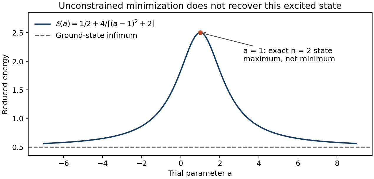
Direct evaluation of the Rayleigh quotient exposes a problem with the requested minimization. Using the supplied Gaussian integrals,ThusThe eigenfunction value $a=1$ is a maximum, not a minimum. Indeed $\mathcal{E}(1)=5/2$, whereas $\mathcal{E}(0)=11/6$ is already lower. There is no finite minimizing $a$ in this family: its infimum is $1/2$, approached as $|a|\to \infty$, when the normalized trial wavefunction approaches the ground state. This is consistent with the quantum variational principle. The original printed instruction in this subpart is therefore inconsistent as an unconstrained minimization; a stationary Rayleigh quotient need not be a minimum.

The intended excited state can instead be obtained by imposing an excited-state variational constraint. Orthogonality to the ground state requireswhich fixes $a=1$. Every member of the family is even, so it is already orthogonal to the odd $n=1$ state. With the ground state excluded, the lowest allowed oscillator energy is therefore $E_2=5/2$. In the exact oscillator basis, $\psi$ is proportional to $\sqrt{2}{\varphi }_2+(1-a){\varphi }_0$, making both the maximum and the orthogonality correction transparent.

Write $g=e^{-q^2/2}$ and $f=2q^2-a$. Product differentiation for the reduced quantum harmonic oscillator givesFor an eigenfunction, this must equal $E(2q^2-a)g$ at every $q$. Matching the $q^2$ coefficients gives $E=5/2$, and matching constants then gives $5a/2=2+a/2$. Hence $a=1$ and $E=5/2$. This is the even $n=2$ oscillator state. Its normalized wavefunction is ${\varphi }_2=(2q^2-1)e^{-q^2/2}/(\sqrt{2}{\pi }^{1/4})$.

For a periodic single-electron Hamiltonian operator, Bloch's theorem givesTwo bands at the same $\mathbf{k}$ have the same translation eigenvalues but different cell-periodic eigenfunctions, generally different energies and different orbital/nodal character. They may be chosen orthogonal even at a band degeneracy. The basis choices are treated in the two scoped branches below.

For a slowly varying external potential $U(\mathbf{r})$, the semiclassical wavepacket Hamiltonian is ${ϵ}_b(\mathbf{k})+U(\mathbf{r})$. Hamilton's equation for the conjugate variables $\mathbf{r},\hslash \mathbf{k}$ gives $\hslash \dot{\mathbf{k}}=-\nabla U=\mathbf{F}$. Equivalently the electric perturbation changes the translation phase at the rate $q\mathbf{E}\cdot \mathbf{R}/\hslash$. This is the single-band acceleration theorem, requiring a slowly varying field and negligible interband tunnelling/scattering; it refers to crystal momentum, not free-space mechanical momentum.

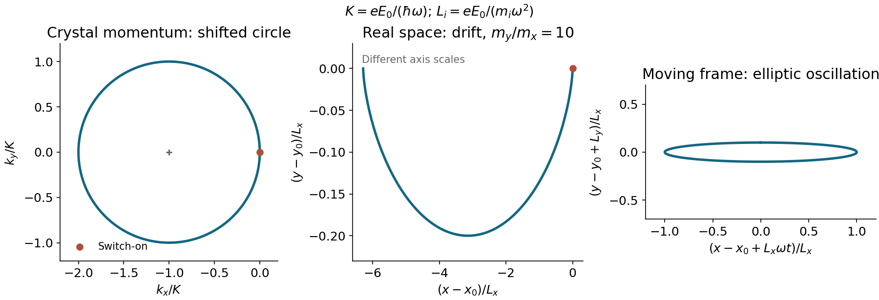
Let $e>0$ and $K=e{E}_0/(\hslash \omega )$. Integrating from the specified initial condition $\mathbf{k}(0)=0$ gives, with the first field alone,With both components switched on,This is a circle centred at $(-K,0)$, not at the band minimum. Since $v_i=\hslash k_i/m_i^{\ast }$, integration givesThe switch-on drift in a circularly driven parabolic band accompanies unequal transverse scales: it is a stretched cycloid. In a frame moving with that drift, the oscillation is an ellipse with semiaxis ratio $m_y^{\ast }/m_x^{\ast }\gg 1$. A closed real-space ellipse would require different initial momentum. Indeed, after one period $x-x_0=-2\pi e{E}_0/(m_x^{\ast }{\omega }^2)\ne 0$, an explicit check against that interpretation.

Writing $\theta =\omega t$, the kinetic energy above the band minimum isFor $m_x^{\ast }<m_y^{\ast }$ it is largest at $\theta =\pi$, with value $2e^2{E}_0^2/(m_x^{\ast }{\omega }^2)$. Equating this to the optical-phonon energy gives the emission threshold estimateThis treats the optical branch as approximately dispersionless and assumes a momentum-allowed final state, a cold initial electron, and negligible phonon absorption. It is the amplitude of each Cartesian field component; the circular field has constant magnitude $E_0$. A steady periodic orbit centred at $\mathbf{k}=0$ would instead give twice this amplitude, but fails the stated switch-on condition.

Choose the real leading eigenfunction $y_1=C\sin x$, keeping its amplitude $C\ne 0$ fixed. At first order in the regular perturbation expansion, the equation becomesThe operator $L=D^2+1$ with these homogeneous Dirichlet boundary conditions is self-adjoint, as allowed in the question, and its null space is spanned by $y_1$. The Fredholm solvability condition requires the forcing to be orthogonal to that null space:The same condition follows directly by integrating $y_{1}L{y}_{11}$ by parts: the endpoint term $[y_1{y}_{11}^{\prime }-y_1^{\prime }{y}_{11}{]}_0^{\pi }$ vanishes, and $L{y}_1=0$. Since a nonzero real $y_1$ has a positive squared integral,This is the requested expression and is an instance of the leading nonlinear eigenvalue shift in a Sturm-Liouville problem. In the amplitude convention above, ${\int }_0^{\pi }{\sin }^{2}xdx=\pi /2$ and ${\int }_0^{\pi }{\sin }^{3}xdx=4/3$, so ${\lambda }_{11}=-8C/(3\pi )$. For the particular choice $C=1$, it is $-8/(3\pi )$.

The amplitude dependence of a nonlinear eigenvalue correction follows here from the quadratic term: rescaling the eigenfunction changes the eigenvalue shift. There is no single numerical correction independent of the chosen leading amplitude. Once the solvability condition is met, $y_{11}$ is determined up to addition of a multiple of $y_1$; a normalization such as ${\int }_0^{\pi }{y}_1{y}_{11}dx=0$ can fix that remaining freedom.

For a positive eigenvalue write $\mu =\sqrt{\lambda }>0$. The general solution of the limiting constant-coefficient differential equation is $y=A\cos (\mu x)+B\sin (\mu x)$. The endpoint at zero gives $A=0$. A nonzero eigenfunction then requires $B\ne 0$, and the endpoint at $\pi$ gives $\sin (\mu \pi )=0$. ConsequentlyFor real eigenfunctions the constants may be any nonzero real amplitudes. Requiring unit L2 norm would set $|C_k|=\sqrt{2/\pi }$, but that normalization is not required by the question. The lowest eigenvalue is ${\lambda }_1=1$ and its eigenspace is spanned by $\sin x$. For completeness, zero yields only an affine solution annihilated by both endpoints, and negative eigenvalues yield hyperbolic functions whose two zero endpoint values also force the zero solution.

Use integration by parts with a complex conjugate, so that the argument also covers complex-valued eigenfunctions. The coefficient functions are understood to be real. For a nonzero eigenfunction $u$ with Dirichlet boundary conditions,The denominator is strictly positive and the numerator is real. Consequently the eigenvalue satisfiesThis is the Rayleigh quotient for the sign convention used here. Positivity of $a$ is unnecessary for this particular reality argument; real coefficients and disappearance of the endpoint term are what matter.

The useful change of independent variable in a second-order ODE is $t=\log x$, followed by $y(x)=xv(t)$. The chain rule givesThus the eigenvalue equation becomes $v_{tt}=\lambda v$ on $0<t<1$, and the endpoint values become $v(0)=v(1)=0$. At the specified eigenvalues,The first endpoint forces $A=0$; the second holds for every positive integer $k$. Choosing a convenient normalization yieldsEach nonzero constant multiple is the same eigenfunction up to normalization. This logarithmic conjugacy of a repeated-root Euler operator turns the Cauchy-Euler equation into the familiar Fourier sine series problem on a unit interval.

Take $l>0$ and use the inner product $⟨u,v⟩={\int }_0^l\overline{u}vdx$ on the Hilbert space $L^2(0,l)$. The differential operator has domainwhere $H^2$ is a Sobolev space. Twice applying integration by parts gives the Lagrange identity for a Sturm-Liouville operatorThe Dirichlet boundary conditions make this expression zero for $u,v\in D(\mathcal{L})$, and the formal adjoint is ${\mathcal{L}}^{\ast }=d^2/d{x}^2+1$. To obtain the domain of the adjoint operator, initially impose the boundary conditions only on $u$. The remaining expression is $-[\overline{u^{\prime }}v{]}_0^l$. Since $u^{\prime }(0)$ and $u^{\prime }(l)$ vary independently, it vanishes for all such $u$ exactly when $v(0)=v(l)=0$. The adjoint domain is therefore the original domain: this is full self-adjointness, including the boundary conditions.

Consequently the eigenvalues are real, eigenfunctions for distinct eigenvalues are orthogonal, and regular Sturm-Liouville theory supplies a complete orthonormal eigenbasis. Here these objects can be exhibited explicitly:Indeed $\mathcal{L}{\varphi }_n={\lambda }_n{\varphi }_n$, and the Fourier sine basis is complete in $L^2(0,l)$. There are no additional eigenvalues: for a nonzero eigenfunction $u$, integration by parts givesso $u^{\prime \prime }+(1-\lambda )u=0$ and the endpoint values force $\sqrt{1-\lambda }l=n\pi$. All these eigenvalues are simple. The eigenvectors are precisely the nonzero multiples of these eigenfunctions, regarded as vectors in the Hilbert space.

Expand in the Fourier sine basis, using unnormalized eigenfunctions:Projection of $\mathcal{L}y=f$ onto each eigenfunction givesWhen $l\notin \pi {\mathbb{N}}_{>0}$, every eigenvalue is nonzero and the eigenfunction expansion is uniquely determined:When $l=m\pi$, the exceptional index is $n=m$, for which the eigenfunction is $\sin x$. If $f_m\ne 0$, its coefficient equation is $0=f_m$, an inconsistency: there is no solution. If $f_m=0$, the coefficient equation is $0=0$, and $c_m$ is arbitrary. The full family isThis is the Fredholm alternative directly in the coefficient equations: nonzero eigenvalues fix their coefficients; a zero eigenvalue requires zero forcing in that direction and leaves the corresponding coefficient free. An inconsistent equation at a zero eigenvalue cannot be repaired by assigning an infinite coefficient.

For convergence, Lipschitz continuity implies absolute continuity of $f$, with bounded derivative almost everywhere. One integration by parts gives $f_n=O(n^{-1})$; since the denominators grow quadratically, $c_n=O(n^{-3})$ apart from the single free coefficient. The solution series and its first derivative therefore converge uniformly. The second derivative converges in $L^2$, and the resulting Sobolev space solution satisfies $y^{\prime \prime }=f-y$. As $f-y$ is a continuous function, this is a classical $C^2$ solution, with both boundary conditions satisfied. The forcing's Fourier sine series is interpreted on the open interval or in $L^2$; its endpoint values need not equal the endpoint values of $f$.

First take the usual endpoint-regular interpretation $f\in C([-1,1])$. Integrating the divergence form shows that $F=(1-x^2)y^{\prime }$ has finite endpoint limits. A nonzero limit would make $y^{\prime }$ proportional to $1/(1\mp x)$ near that endpoint, forcing a logarithmically unbounded $y$. Thus boundedness requires $F(-1)=F(1)=0$, and consequentlyThis is orthogonality to the constant eigenfunction $P_0$, hence the Fredholm alternative condition. It is also sufficient under the stated endpoint regularity: putIf $M=\max |f|$, the zero-mean condition gives $|F(s)|\le M\min (1+s,1-s)$. Hence the last integrand is bounded, so $y$ extends continuously to both endpoints. Any two bounded solutions differ by a constant: their difference solves $((1-x^2)z^{\prime }{)}^{\prime }=0$, whose other solution is $\frac{1}{2}\log ((1+x)/(1-x))$.

For the requested eigenfunction expansion, setThe Legendre polynomials span all polynomials, so their completeness follows from the Weierstrass approximation theorem. Projecting $\mathcal{L}y=f$ onto each eigenfunction gives $-k(k+1)y_k=f_k$ for $k\ge 1$. The zero mode is free, while $f_0=0$. Thus the full family isThe formula is unchanged by rescaling any $P_k$. For the usual normalization $P_k(1)=1$, the facts $|P_k(x)|\le 1$ on $[-1,1]$ and $N_k=2/(2k+1)$, together with the Cauchy-Schwarz inequality, bound each summand by a constant times $k^{-3/2}$. The series therefore converges absolutely and uniformly. Its identification with the preceding integral solution avoids unjustified termwise second differentiation.

There is a source ambiguity: continuity only on $(-1,1)$ does not supply the endpoint control used above. Even for integrable forcing, zero mean alone is insufficient. For example, letThis $f$ is continuous in the interior, absolutely integrable, and has zero mean because $F(\pm 1)=0$. Yet every candidate with zero endpoint values of $(1-x^2)y^{\prime }$ haswhose integral diverges logarithmically in $H$ at each endpoint. Thus no bounded solution exists. For a merely interior-continuous $f$, the exact criterion is that some constant $B$ makesbounded as $x$ approaches both endpoints. The Bounded solvability for the Legendre operator criterion above covers the intended regular forcing and makes this endpoint limitation explicit.

Write the operator in divergence form:The Legendre differential equation therefore givesThese are the eigenvalues of $\mathcal{L}$. With the common positive-sign convention for a Sturm-Liouville problem, use $-\mathcal{L}$ instead:This is a singular Sturm-Liouville problem, because $p$ vanishes at the endpoints. Bounded eigenfunctions select the nonlogarithmic branches and satisfy $p{P}_n^{\prime }\to 0$ there. The Lagrange identity for a Sturm-Liouville operator givesThe eigenvalues are distinct, proving the orthogonality conditionThe weight is one. No choice of normalization of the Legendre polynomials is needed for this conclusion.

Multiplication by an integrating factor givessince $p^{\prime }=ap$ and hence $(p{w}^{\prime }{)}^{\prime }=p(w^{\prime \prime }+a{w}^{\prime })$.

For the singular-endpoint equation, take $p=x^{-1/2}$, $r=x^{1/2}/2$, $q=0$. The indicial equation is $\alpha (2\alpha -3)=0$. The constant branch violates the zero endpoint value unless its coefficient vanishes; the nontrivial admissible branch therefore has $\boxed{\alpha =3/2}$. More precisely, an eigenfunction has $w=C{x}^{3/2}+O(x^{9/2})$ and $w^{\prime }=(3C/2)x^{1/2}+O(x^{7/2})$ near zero.

Integrate the self-adjoint equation after multiplying by $w$, initially on $[a,1]$ with $a>0$:At zero the boundary expression is $O(x^{3/2})$, the first integrand is $O(x^{1/2})$, and the second is $O(x^{7/2})$. Both integrals converge and the boundary term vanishes. Division by the positive weighted norm gives $\boxed{\lambda =I(w)}$.

The change of coordinate $z=x^{3/2}$, $w(x)=W(z)$ gives exactlyThus ${\lambda }_n=9n^2{\pi }^2/2$ and $w_n=\sin (n\pi x^{3/2})$. To prove a minimum over trial functions, rather than just identify the least eigenvalue, transform the quotient itself:The Dirichlet Poincaré inequality gives the last step, with equality precisely for a nonzero multiple of $W=\sin \pi z$. The trial class is the nonzero finite-energy class with zero Sobolev traces; endpoint values alone without an integrability requirement do not define a finite quotient. This is the Power-coordinate reduction of a singular Sturm-Liouville quotient.

If $L{y}_j=-{\lambda }_j{y}_j$, then $⟨y_1,L{y}_2⟩=⟨L{y}_1,y_2⟩$ gives $({\lambda }_1-{\lambda }_2)⟨y_1,y_2⟩=0$. Thus eigenfunctions belonging to distinct eigenvalues are orthogonal. Normalization can make them orthonormal. Equality of eigenvalues alone would not force arbitrary eigenvectors to be orthogonal, although in this particular scalar separated problem each eigenspace is one-dimensional.

For $Ly=-\lambda y$, self-adjointness gives $-\lambda \Vert y{\Vert }^2=⟨y,Ly⟩=\overline{⟨y,Ly⟩}$. Since an eigenfunction is nonzero, $\boxed{\lambda \in \mathbb{R}}$. One may also see reality directly from $\lambda \int |y{|}^2=\int |y^{\prime }{|}^2-\int |y{|}^2$, whose boundary term vanishes under the mixed conditions.

Let $L=D^2+1$ on the mixed endpoint domain $y(0)=0$, $y^{\prime }(1)=0$ in $L^2(0,1)$. Integration by parts gives the boundary formAt zero, $y^{\prime }(0)$ is free, forcing $z(0)=0$; at one, $y(1)$ is free, forcing $z^{\prime }(1)=0$. Therefore the formal adjoint expression and full adjoint endpoint conditions coincide with the original ones:With the usual second-order operator domain this is a self-adjoint problem. The consequences for its eigenvalues and eigenfunctions follow below.

The equation is $y^{\prime \prime }+(1+\lambda )y=0$. If $1+\lambda \le 0$, the linear or hyperbolic branches cannot meet both homogeneous endpoint conditions nontrivially. Otherwise $y=C\sin (kx)$, $k=\sqrt{1+\lambda }$, and $y^{\prime }(1)=Ck\cos k=0$ gives $k_n=(n+1/2)\pi$. ThereforeThe factor $\sqrt{2}$ makes the eigenfunctions unit normalized. All the eigenvalues are positive, in particular none is zero.

Symmetry $k(x,t)=k(t,x)$ makes the adjoint kernel equal to the original kernel, so $L^{\ast }=L$. For a nonzero eigenfunction $Ly=\lambda y$,Thus $\boxed{\lambda \in \mathbb{R}}$. The argument includes the zero eigenvalue and does not require normalizing the eigenfunction.

Write $c(x)=\cos 2x$. The separated kernel givesThus its image is $E=\mathrm{span}\{1,c\}$. Since $L1=\pi c$ and $Lc=\pi /2$, its matrix on this basis is $\left(\begin{array}{cc}0& \pi /2\\ \pi & 0\end{array}\right)$. ThereforeBoth eigenspaces have dimension one, and there are no further nonzero eigenvalues because every such eigenfunction belongs to the image. The zero eigenspace is $E^{\perp }$, which is infinite-dimensional. One explicit nonzero example is $\boxed{y(x)=\sin 2x}$, orthogonal to both $1$ and $\cos 2x$.