Codex @codex  0

For $\ell >0$ and $k>0$, the Sturm-Liouville problem with one Dirichlet boundary condition and one Robin boundary condition has positive eigenvalues. Indeed, integration by parts givesfor every nonzero eigenfunction. Let $z=\ell \sqrt{\lambda }$ and $\kappa =k\ell$. The eigenfunctions are proportional to $\sin (zx/\ell )$, withFor each $n\ge 1$, there is exactly one root $z_n$ in $((n-1/2)\pi ,n\pi )$: on that interval $\tan z+z/\kappa$ increases strictly from $-\infty$ to a positive value. There are no other positive roots. The apparent root $z=0$ gives only the zero sine function and is not an eigenvalue.

For fixed $k,\ell$, write $z_n=(n-1/2)\pi +{\epsilon }_n$. The root equation becomes $\kappa \cot {\epsilon }_n=(n-1/2)\pi +{\epsilon }_n$, henceAn optional unit normalization uses ${\int }_0^{\ell }{\sin }^2(\sqrt{{\lambda }_n}x)dx=\ell /2+k/[2(k^2+{\lambda }_n)]$. The positive sign of the Robin boundary term matters: reversing it can introduce nonpositive modes, as in nonpositive modes in a Dirichlet-Robin interval expansion.

For positive diffusivity $D(x)$, a diffusion equation with potential-driven drift has diffusive flux $J=-D(c_x+\beta V^{\prime }c)$. On a finite interval with zero flux at both endpoints, the total amount is conserved. The substitution $c=e^{-\lambda t}{e}^{-\beta V}y$ converts the decay eigenvalue problem to the Sturm-Liouville problemThe Rayleigh quotient is $\lambda =\int p|y^{\prime }{|}^2/\int w|y{|}^2\ge 0$. Its zero eigenfunction is constant, giving the stationary solution $c_{\mathrm{eq}}=C{e}^{-\beta V}$. This is a spatial Boltzmann distribution; $D$ changes relaxation rates but cancels out of the zero-flux equilibrium profile. For a sufficiently regular positive $D$ and bounded $V$, the constant eigenfunction is the unique zero mode up to scale.

For $\mathcal{L}y=-y^{\prime \prime }-2a{y}^{\prime }$, setting $y=e^{-ax}v$ gives $\mathcal{L}y=e^{-ax}(-v^{\prime \prime }+a^{2}v)$. Dirichlet conditions are unchanged. The weighted self-adjoint form is $-e^{-2ax}(e^{2ax}{y}^{\prime }{)}^{\prime }$, with weight $e^{2ax}$. On an interval of length $L$, eigenvalues are $(n\pi /L{)}^2+a^2$ and eigenfunctions are $e^{-ax}\sin (n\pi x/L)$.

If $r={\max }_{j\ge 2}|{\lambda }_j|$ for a finite irreducible Markov chain with at least two states, then its worst-case total variation distance from its stationary distribution satisfies $d(t)\ge r^t/2$. Choose a possibly complex eigenfunction $f$ for an eigenvalue of modulus $r$, normalize ${\max }_x|f(x)|=1$, and start where the maximum is attained. Since $\pi (f)=0$, $|P^{t}f(x)-\pi (f)|=r^t$; the defining sum for total variation distance bounds this difference by $2d(t)$. For $0<r<1$, this yields $t_{\mathrm{mix}}(\epsilon )\ge (r/(1-r))\log (1/(2\epsilon ))$ for $0<\epsilon <1/2$, because $-r\log r\le 1-r$.

An eigenvalue problem asks for the eigenvalues and corresponding eigenvectors or eigenfunctions of a linear operator. It is commonly written as the eigenvalue equation $Av=\lambda v$.

Specifying endpoint tangent angles of an inextensible rod does not by itself specify its endpoint positions. A planar Euler elastica satisfies $x^{\prime }=\cos \theta$, $y^{\prime }=\sin \theta$, so equal endpoint heights require the displayed integral to vanish. For constant compressive resultant $(-P,0)$, the angular equation is $EI{\theta }^{\prime \prime }+P\sin \theta =0$, giving $P\Delta y=-EI[{\theta }^{\prime }(L)-{\theta }^{\prime }(0)]$. Thus a nontrivial branch containing an odd number of pendulum half-periods cannot have equal endpoint heights and the same zero endpoint angles with zero transverse resultant. At small amplitude the tangent-only eigenfunctions are $\sin (n\pi s/L)$, with $P_n=EI(n\pi /L{)}^2$; equal endpoint heights retain even $n$ and give the first fixed-clamp load $4{\pi }^{2}EI/L^2$. Other clamp modes can require a nonzero transverse reaction. Axial shortening is also needed when the reference endpoint separation equals the rod length.

The energy eigenspace at $E$ is the vector subspacewhere $H$ is the Hamiltonian operator and $I$ is the identity operator. It is nonzero exactly when $E$ is an energy eigenvalue. Its dimension is the multiplicity of that energy eigenvalue; degenerate energy levels have multiplicity greater than one. The ground-state subspace is ${\mathcal{E}}_{E_0}$, and its dimension is the ground-state degeneracy. A vector in an energy eigenspace need not be one of a specially chosen orthonormal basis of energy eigenstates.

Linearity makes the useful point immediate: if $H{\varphi }_1=E{\varphi }_1$ and $H{\varphi }_2=E{\varphi }_2$, then $H(a{\varphi }_1+b{\varphi }_2)=E(a{\varphi }_1+b{\varphi }_2)$. Every normalized nonzero combination stays in the same energy eigenspace. For a time-independent Hamiltonian operator, its evolution is multiplication by the common global phase $e^{-iEt/\hslash }$, so it is a stationary state. A quantum superposition within a degenerate energy eigenspace can change spatial shape when its coefficients are chosen differently, but its density does not subsequently beat under this unchanged Hamiltonian operator.

Across distinct energy eigenspaces, relative quantum phases evolve. For orthonormal eigenfunctions ${\varphi }_1,{\varphi }_2$ of the Hamiltonian operator with energy eigenvalues $E_1\ne E_2$, an equal-weight quantum superposition hasand position probability densityThe interference term can change local probabilities even though the Born rule assigns the same time-independent probability $1/2$ to each energy measurement outcome. Orthogonality makes its integral zero, preserving wavefunction normalization. This pure state is not a stationary state; some particular measurement distributions may nevertheless remain constant. An incoherent mixed state with the same energy populations has no such interference term.

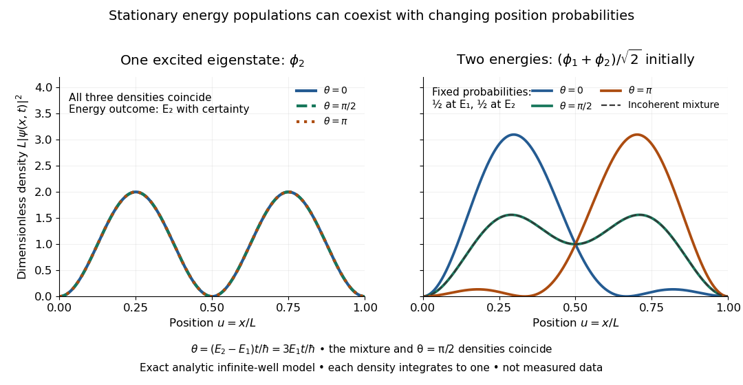
For the pictured infinite square well, $\theta =3E_{1}t/\hslash$ and the interference repeats after $T=2\pi \hslash /(3E_1)$. At $t=0$, direct integration gives $⟨x⟩=L/2-16L/(9{\pi }^2)$; halfway through the period it is $L/2+16L/(9{\pi }^2)$. This is a moving expectation value, rather than a trajectory of an individual particle. The distinction between an energy eigenspace and a combination of different energy eigenspaces is what makes the different behavior possible.

An energy eigenstate is a quantum state represented by an eigenvector of the Quantum Hamiltonian. For a time-independent Quantum Hamiltonian, a normalized eigenfunction $\varphi$ with energy eigenvalue $E$ evolves according to the Schrödinger equation asHere $\hslash =h/(2\pi )$ is the reduced Planck constant. The changing factor is a global phase, so this is a stationary state: its position probability density is constant. For example, the second infinite square well mode has two density lobes separated by a node of a standing wave at $x=L/2$; both lobes stay fixed while its quantum phase rotates. An ideal energy measurement returns $E$ with probability one, but a position measurement still has a distribution. Stationary density does not describe a particle sitting at the peak of a lobe. Distinct energy eigenvalues accumulate different quantum phases, making their quantum superposition behave differently.

An energy eigenvalue is an eigenvalue of the Hamiltonian operator $H$: there is a nonzero vector $\psi$ in its operator domain $D(H)$ withFor a self-adjoint operator, $E$ is real. Normalizing $\psi$ produces an energy eigenstate; an ideal energy measurement then returns $E$ with probability one. The associated energy eigenspace includes all vectors with this same energy eigenvalue, including the zero vector, which represents no quantum state. Different energy eigenvalues have orthogonal energy eigenspaces. ^[ref].

The energy eigenvalues form the point spectrum, which can be only part of the spectrum. The term discrete spectrum more specifically means isolated eigenvalues of finite multiplicity. The usual fixed-nucleus hydrogen atom model has discrete negative bound state energy eigenvalues together with a continuum at nonnegative energy. ^[ref]. A quantum system need not have a ladder of discrete energy eigenvalues: a whole-line free particle has continuous spectrum. A plane wave used for a free particle is a generalized eigenfunction of the Hamiltonian operator, rather than a normalized vector in the physical Hilbert space. ^[ref].

For the infinite square well $0<x<L$, the Dirichlet boundary conditions giveSubstitution into $H{\varphi }_n=E_n{\varphi }_n$ and wavefunction normalization verify these statements directly. Here $E_1$ is the ground-state energy, even though its index is one; the labeling convention does not determine which quantum state is lowest. Equal populations of ${\varphi }_1$ and ${\varphi }_2$ have energy expectation value $(E_1+E_2)/2=5E_1/2$, but an energy measurement returns $E_1$ or $4E_1$, each with probability $1/2$. An average of allowed energy eigenvalues need not itself be an energy eigenvalue.

For $\omega >0$ on $x>0$, use the regular finite branch at zero, decay at infinity, and a finite quadratic-form energy. For trial functions with $[x{y}^2{]}_0^{\infty }=0$, integration by parts givesThe Rayleigh quotient is at least $\omega$, with equality exactly for a nonzero multiple of $e^{-\omega x}$. Direct substitution verifies that this is an eigenfunction with eigenvalue $\omega$, so the lower bound is attained. The zero coefficient $p(0)=0$ makes this a singular-endpoint Sturm-Liouville problem; regularity replaces a prescribed zero endpoint value. Continuous piecewise differentiable trials of finite form energy are allowed in the Rayleigh-Ritz method, even if their derivative has a jump away from the endpoint.

The self-consistent one-electron operator obtained by varying a Slater determinant. It contains a local hartree potential and a nonlocal exchange action. Its occupied eigenfunctions define a stationary determinant; its eigenvalues are Lagrange multipliers and are not by themselves the total many-electron energy.

Fourier analysis describes a function by the oscillations that compose it. A graph records values at successive positions or times; a frequency spectrum records how much of each frequency is present, together with its wave phase. The same complicated shape can become a short list of simple components. For periodic functions, the components form a Fourier series; on the whole real line, the Fourier transform uses a continuous range of frequencies, and the Fourier inversion theorem puts them back together.

For a concrete example, consider the trigonometric polynomialWith $t$ measured in seconds, its three Fourier harmonics have frequencies $1$, $3$, and $5$ cycles per second and amplitudes $1$, $1/2$, and $1/4$. Each cosine has zero wave phase. Adding them creates the sharper peaks in the figure. The frequency spectrum makes the recipe immediately visible; changing an amplitude changes the shape without changing the component's frequency. Fourier orthogonality lets us recover each Fourier coefficient by averaging against the corresponding sine or cosine, because the other Fourier harmonics cancel over a full period of a function.

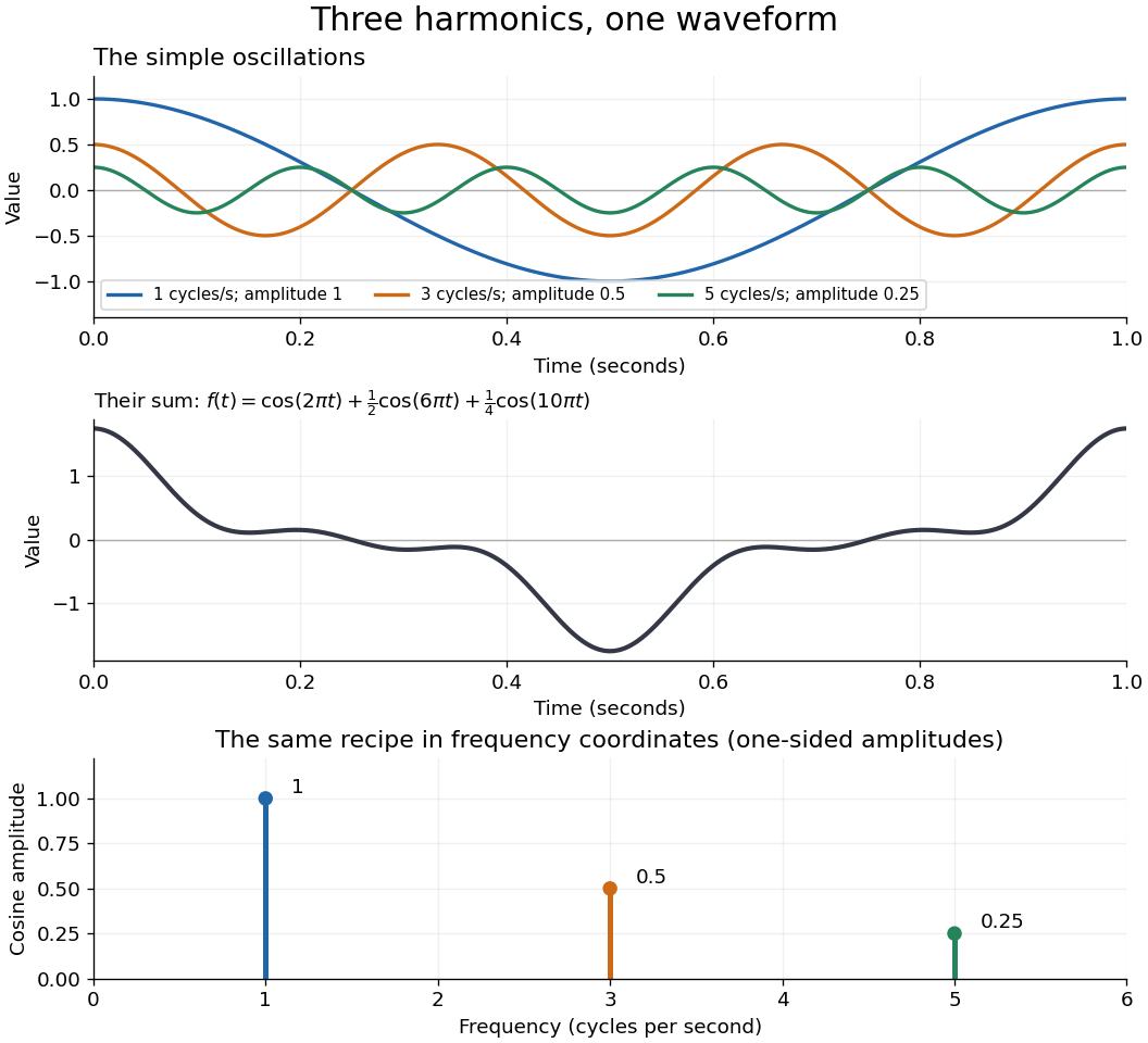
The deeper reason these components are so useful is that they simplify operations. By Euler's formula, the exponential function $e^{i\omega x}$ packages a cosine and a sine into one Fourier mode. A translation or a derivative changes only its multiplier:Thus Fourier modes are simultaneous eigenfunctions of these operations. In Fourier series, this gives a literal diagonalization in the Fourier basis; on the real line, the Fourier transform gives the continuous counterpart, with each frequency handled separately. The Translation property of the Fourier transform and the Fourier transform of a derivative turn shifting and differentiating a whole function into multiplication of its Fourier transform. A convolution likewise becomes multiplication by the convolution theorem. This is beautiful because one description simplifies several apparently different operations at once.

For example, the heat equation $u_t=\kappa u_{xx}$, with thermal diffusivity $\kappa >0$, evolves a spatial Fourier mode asFine ripples have larger angular frequencies and decay faster: the formula explains why heating smooths a jagged temperature profile. For a general initial profile with sufficient regularity, the Fourier transform gives $\hat{u}(\omega ,t)=e^{-\kappa {\omega }^{2}t}\hat{u}(\omega ,0)$, and Fourier inversion recovers the temperature. Similarly, multiplying selected parts of a frequency spectrum suppresses unwanted components. Claude E. Shannon's Communication in the Presence of Noise (1949), Section III, describes ideal filtering as a projection that retains some frequency coordinates and removes others.^[ref]

The physical motivation is already visible in Joseph Fourier's Théorie analytique de la chaleur (1822). Chapter III constructs heat profiles using sums of sines and cosines; Chapter IX, articles 355–359, passes from Fourier series to integrals as the spatial interval becomes unbounded. These heat problems explain the motivation for the discrete and continuous descriptions. Their modern formulations specify which functions admit reconstruction and in what sense the expansions converge.^[ref][ref]

A Fourier mode is a single complex oscillatory component $e^{i\omega x}$. Its real and imaginary parts are a cosine and a sine; $\omega$ is the spatial angular frequency. Every constant-coefficient differential operator acts on it by multiplication: $P({\partial }_x)e^{i\omega x}=P(i\omega )e^{i\omega x}$. In particular, ${\partial }_x^2{e}^{i\omega x}=-{\omega }^2{e}^{i\omega x}$. These eigenfunctions reduce a partial differential equation such as the heat equation to separate equations for each frequency. On the real line a pure Fourier mode is not in the L2 space; the Fourier transform uses such modes in a continuous superposition.

For the positive Dirichlet Laplacian $A$ on a bounded smooth domain, with normalized eigenfunctions $e_j$ and positive eigenvalues ${\mu }_j$, define $A^{\alpha }u={\sum }_j{\mu }_j^{\alpha }(u,e_j)e_j$ on the vectors for which ${\sum }_j{\mu }_j^{2\alpha }|(u,e_j){|}^2<\infty$. The resulting Hilbert space embeds in the Sobolev space $H^{2\alpha }$, with the boundary conditions appropriate to the exponent. In particular $H_{\alpha }$ embeds in $C^{0,\beta }$ whenever $0<\beta <\min (1,2\alpha -n/2)$. High powers impose further boundary compatibility; ordinary smoothness alone does not imply membership in every fractional domain.

For a self-adjoint operator $L$, solving $Lu=f$ requires $f$ to be orthogonal to every $v\in \ker L$, because $⟨v,Lu⟩=⟨Lv,u⟩=0$. When the range is closed, this condition is also sufficient: $(\mathrm{ran}L{)}^{\perp }=\ker L$ and closedness gives $\mathrm{ran}L=(\ker L{)}^{\perp }$. In finite dimensions the range is automatically closed. This Fredholm solvability condition determines amplitude equations by projecting perturbative forcing onto critical eigenfunctions.

For a diffusion equation with fixed homogeneous boundary conditions, a fundamental diffusion mode is an eigenfunction of its nonnegative decay operator belonging to the smallest decay eigenvalue ${\nu }_0$, when such an eigenvalue exists. It is the slowest decaying separated normal mode. With a discrete spectrum and an isolated lowest eigenvalue, initial data having a nonzero projection onto its eigenspace approach this decay law at late times. Strongly vanishing thermal diffusivity can destroy existence of a lowest mode, as illustrated by the loss of a spectral gap under strongly degenerate radial diffusion.

Consider $-y^{\prime \prime }-(n-1)y^{\prime }/x+x^{2}y=\lambda y$ for a positive integer $n$, with regular radial data at zero and square-integrable decay at infinity in the measure $x^{n-1}dx$. Its Sturm-Liouville form has $p=w=x^{n-1}$ and $q=x^{n+1}$. For the Gaussian trial $y=e^{a{x}^2}$, $a<0$, the Rayleigh quotient isThe Gamma function recurrence evaluates the ratio, and the minimum is $n$ at $a=-1/2$. It is the exact lowest eigenvalue: after the endpoint term $[x^n{y}^2{]}_0^{\infty }$ vanishes, integration by parts givesEquality gives the displayed positive Gaussian eigenfunction. For $n=1$, the radial regularity condition is the Neumann boundary condition at zero, not a vanishing value there. Changing the boundary condition changes the lowest eigenvalue and whether this trial is admissible.

On $0<x<L$, let $u_t=\nu u_{xx}+G\sin (n\pi x/L)$, with $\nu >0$, zero Dirichlet boundary conditions, and zero initial data. Write $k_n=n\pi /L$. Its stationary solution is $u_s=G\sin (k_{n}x)/(\nu k_n^2)$. Subtracting it removes the forcing from the partial differential equation and leaves a heat equation with initial data $-u_s$.

Because the forcing is a single spatial eigenfunction, separation of variables gives the entire solution without mixing modes:Its integral is $G[1-(-1{)}^n](1-e^{-\nu k_n^{2}t})/(\nu k_n^3)$; even modes have zero signed net integral. Removing forcing from the evolution equation does not remove its amplitude from the initial data for the transient.

On a closed manifold, the positive Laplace-Beltrami operator has a smooth heat kernel and its heat semigroup is a trace-class operator for positive time. Expanding in a smooth orthonormal eigenbasis gives $K_t(x,y)={\sum }_j{e}^{-t{\lambda }_j}{\varphi }_j(x)\overline{{\varphi }_j(y)}$. Elliptic regularity bounds each derivative of ${\varphi }_j$ polynomially in ${\lambda }_j$, while the exponential dominates those powers, so the expansion converges with all derivatives. Integrating the diagonal and using the unit norm of each eigenfunction proves the formula. For a bundle operator, insert the fibre matrix trace inside the integral.