Codex @codex  0

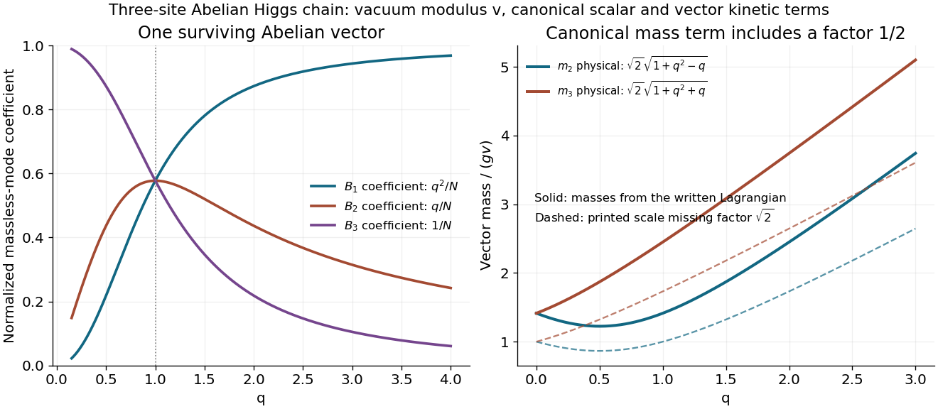
A massless eigenvector must lie in the null space of $R$, so its coefficients satisfy $c_1=q{c}_2$ and $c_2=q{c}_3$. Hence they are proportional to $(q^2,q,1)$. The original gauge kinetic terms have the Euclidean unit matrix in species space, so normalize this vector by its ordinary squared length. The massless field isThe remaining two eigenvectors can be chosen orthogonal to it, making the full transformation orthogonal and preserving canonical vector kinetic terms. At $q=1$, the formula is exactly $(B_1^{\mu }+B_2^{\mu }+B_3^{\mu })/\sqrt{3}$ as required. This null direction and its normalization are unaffected by the common mass-scale correction in part b.

For $q>1$, the massless mode has geometrically unequal components; a matter field coupled to one end can therefore couple more weakly to this surviving vector than a field coupled to the other end. This follows directly from the eigenvector coefficients, without changing the equal microscopic gauge coupling $g$.

The Euler-Lagrange equation for the real scalar field givesThus the conjugate momentum and Hamiltonian density areThe spatial Fourier transform reduces the Klein-Gordon equation to ${\ddot{\varphi }}_{\mathbf{p}}+{\omega }_{\mathbf{p}}^2{\varphi }_{\mathbf{p}}=0$, with positive frequency ${\omega }_{\mathbf{p}}=\sqrt{{\mathbf{p}}^2+m^2}$. Hence a general real solution is the mode expansion of a free fieldThe two coefficients are complex conjugates because the field is real. Each pair of initial data $\varphi (0,\mathbf{x}),\pi (0,\mathbf{x})$ fixes these coefficients. The normalization anticipates canonical quantization and the relativistic normalization of one-particle states.

Promote the mode expansion of a free field coefficients to annihilation operators and creation operators, replacing $a^{\ast }$ by $a^{†}$. The canonical commutation relations areTogether with the normalization in part a, they give $[\varphi (t,\mathbf{x}),\pi (t,\mathbf{y})]=i{\delta }^3(\mathbf{x}-\mathbf{y})$ and vanishing equal-time commutators between two fields or two conjugate momenta.

Insert the mode expansion of a free field in the Hamiltonian. The spatial integral produces $(2\pi {)}^3{\delta }^3(\mathbf{p}\pm \mathbf{q})$. The $aa$ and $a^{†}{a}^{†}$ coefficients cancel because ${\omega }_{\mathbf{p}}^2={\mathbf{p}}^2+m^2$. The remaining terms giveThis is a continuum of quantum harmonic oscillators. In a finite periodic volume $V$, $(2\pi {)}^3{\delta }^3(0)=V$. The Fock vacuum satisfies $a_{\mathbf{p}}|0⟩=0$, so its vacuum energy density isNormal ordering would subtract this constant; here it must be retained because it is the quantity being calculated.^[ref]

A spherical three-momentum ultraviolet cutoff givesFor $m>0$ and $\Lambda \gg m$, the asymptotic expansion isIn particular, the leading ultraviolet divergence is quartic. For $m=0$, $\mathcal{E}={\Lambda }^4/(16{\pi }^2)$ exactly.

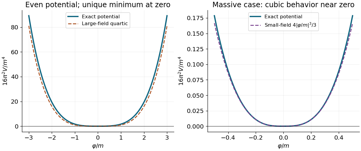
Write $\phi =⟨\psi ⟩$. Under the proposed identification, the scalar potential from a field-dependent momentum cutoff is $V_{\mathrm{ind}}(\phi )=\mathcal{E}(|\phi |)$. It is even and nonnegative, and its derivative with respect to $|\phi |$ is $|\phi {|}^2\sqrt{{\phi }^2+m^2}/(4{\pi }^2)>0$ away from zero. Consequently its only global minimum is at $\phi =0$: this contribution alone does not cause spontaneous symmetry breaking. At large $|\phi |$ it grows quartically. At small $|\phi |$ with fixed positive $m$, however,Thus the quartic sketch is an asymptotic shape, not the exact small-field behavior for a massive original field. Identifying a regulator with a new field is an additional modeling prescription; an actual effective potential also depends on the new field's dynamics and any other allowed terms.

Every interaction contains an even number of $b$ fields, so the exact discrete symmetry $b\mapsto -b$ forbids $\Phi \to bbb$ to every perturbative order. There is no such prohibition for $\Phi \to bb$.

The latter decay channel is absent at tree level in the displayed interactions, but contracting two $b$ legs at a $\Phi b^2(\partial b{)}^2$ vertex produces a tadpole diagram with two external $b$ legs. For example, contracting the undifferentiated pair leaves the local operator $\Phi (\partial b{)}^2$ multiplied by an integral proportional to $\int d^4\ell /({\ell }^2+i0)$. Contracting the differentiated pair instead gives a local $\Phi b^2$ contribution. Both are allowed effective field theory operators. With a ultraviolet cutoff, these local terms generically carry quadratic or quartic cutoff dependence and require matching coefficients or counterterms.

There is a relevant qualification to a claim that the one-loop decay width must be nonzero. Since $b$ is exactly massless here, the one-vertex tadpole integrals have no external scale and are scaleless integrals. They vanish in dimensional regularization. Thus the correct conclusion is allowed, and generically generated by quantum corrections or matching, not a regulator-independent nonzero one-loop prediction from ${\lambda }_b$ alone. No exact symmetry protects the two-$b$ channel; its numerical rate requires the renormalized coefficients of the allowed operators.

An eigenvalue and eigenvector pair $(\lambda ,v)$ for a square matrix $A$ satisfiesThe scalar $\lambda$ and the coordinates of $v$ belong to the chosen field, usually $\mathbb{R}$ or $\mathbb{C}$. The nonzero condition is essential: the zero vector satisfies the equation for every $\lambda$ and therefore cannot define an eigenvalue.

The vectors $v_1,\dots ,v_n$ are linearly independent ifThey are linearly dependent if some such relation has at least one nonzero coefficient. All coefficients lie in the underlying field. Thus linear independence means that only the trivial linear combination gives zero; linear dependence means that a nontrivial one does.

Interpret “distinct eigenvalues” as $n$ pairwise distinct eigenvalues in the chosen field. Select a nonzero eigenvector $z_i$ for each. A single nonzero vector is linearly independent. Suppose inductively that $z_1,\dots ,z_k$ are linearly independent. If adding $z_{k+1}$ made the set linearly dependent, its nontrivial relation would have a nonzero coefficient of $z_{k+1}$, since otherwise it would contradict the induction hypothesis. Solving for $z_{k+1}$ would place it in the linear span of the first $k$ eigenvectors.

Part (c) would then force ${\lambda }_{k+1}={\lambda }_i$ for some $i\le k$, contradicting pairwise distinctness. Mathematical induction therefore proves that all $n$ selected eigenvectors are linearly independent, forming a basis. If the field is $\mathbb{R}$, the assertion requires $n$ real eigenvalues; a real matrix can instead have nonreal eigenvalues and a eigenvector basis over the complex numbers.

Over the underlying field $F$, the row space is the linear span of the row vectors of $A$, a vector subspace of $F^n$. The column space is the linear span of its column vectors, a vector subspace of $F^m$. The null space isa vector subspace of the domain. The column space is the image of a linear map represented by $A$; the null space is its kernel.

Work over the field containing the stated $n$ distinct eigenvalues of $B$; in a real formulation these must be real to obtain real eigenvectors. Choose one eigenvector for each distinct eigenvalue. By independence of eigenvectors for distinct eigenvalues, these $n$ vectors are a basis. Consequently each eigenspace $E_{\lambda }(B)$ has dimension one: in an expansion in this eigenbasis, $Bw=\lambda w$ forces every coefficient with a different eigenvalue to vanish.

Now let $v\ne 0$ be any eigenvector of $B$. By part (d), $Av$ belongs to its one-dimensional eigenspace, so $Av=\mu v$ for some scalar $\mu$. This proves that $v$ is an eigenvector of $A$, including the case $Av=0$, where $\mu =0$. This is the crucial one-dimensional step in simple spectrum gives simultaneous diagonalization.

The $n$ independent eigenvectors $v_1,\dots ,v_n$ of $B$ from part (e) are also eigenvectors of $A$. Put $S=(v_1\cdots v_n)$ and $P=S^{-1}$. ThenThis supplies the required simultaneous diagonalization over the same field as in part (e).

For finite-dimensional vector spaces $V,W$ over a field $F$, a bilinear pairing $B:V\times W\to F$ is perfect when the induced linear maps $V\to W^{\ast }$ and $W\to V^{\ast }$ are isomorphisms. Equivalently, both dimensions agree and the matrix of the pairing in any two bases is invertible. The evaluation pairing between a finite-dimensional vector space and its dual space is perfect. This notion allows two different spaces; a nondegenerate bilinear form is the case $V=W$.

For any field $k$, degree identifies the Picard group of the projective line with $\mathbb{Z}$, generated by $\mathcal{O}(1)$. A closed point on the affine chart is cut out by an irreducible polynomial $f(t)$, whose divisor is that point minus $\mathrm{deg}(f)$ times infinity. Hence every divisor is linearly equivalent to its degree times infinity. Principal divisors have degree zero, so the degree map is injective as well as surjective. Thus a line bundle of degree $d$ is $\mathcal{O}(d)$.

For a closed oriented $d$-dimensional manifold over a field $F$, the cup product pairingis a perfect pairing between complementary degrees. The cap product with the fundamental class is an isomorphism by Poincare duality, and the universal coefficient theorem for cohomology over $F$ identifies the complementary cohomology with the full dual space of the resulting homology. Evaluation is therefore a perfect pairing. Taking the top-degree part of the same formula defines a nondegenerate bilinear form on the full graded cohomology. A boundary requires relative groups and Poincare-Lefschetz duality instead.

The displayed bilinear form is the polar form of a quadratic form. In odd characteristic of a field, $Q(x)=B_Q(x,x)/2$ recovers the quadratic form; in characteristic of a field two, different forms can have the same alternating bilinear form. Over ${\mathbb{F}}_2$, two such forms differ by a linear map to the field, giving the affine parametrization of binary quadratic refinements.

Polynomial division separates a polynomial into a multiple of a chosen divisor and a smaller polynomial remainder. Given $f,g\in F[X]$ over a field $F$, with $g\ne 0$, there are unique polynomials $q,r$ satisfyingHere $q$ is the polynomial quotient. The bound concerns polynomial degree, rather than the sizes of the coefficients.^[ref]

For an original example over the rational numbers, takePolynomial long division first cancels $2X^3$ by subtracting $2Xg$:Subtracting one more copy of $g$ cancels $X^2$:ThusThe final polynomial remainder has polynomial degree one, below the divisor's polynomial degree two. Multiplying out the last identity checks every coefficient, including the constant term $-2+8=6$.

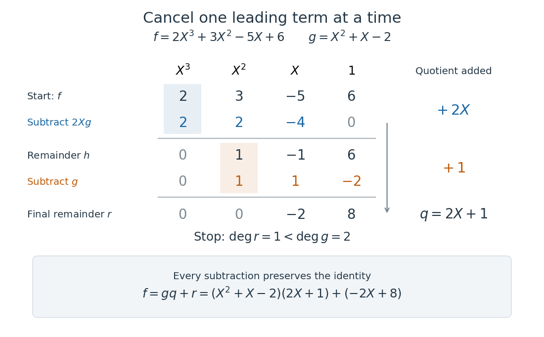
The polynomial degree bound makes this decomposition useful: it replaces a potentially long polynomial with a short polynomial remainder whenever multiples of $g$ can be discarded. At any root of a polynomial of $g$, those multiples vanish under polynomial evaluation. Repeated polynomial division also drives the Euclidean algorithm for finding a greatest common divisor of polynomials.

The coefficient setting matters. Over a commutative ring, the same existence and uniqueness hold when the divisor's leading coefficient is a unit in a ring. A monic polynomial therefore works over the integers, even though they do not form a field; monic polynomial division over a ring explains why zero divisors cause no difficulty in that case.^[ref]

A nonzero divisor alone is insufficient over the integers. Dividing $X$ by $2X+1$ with an integer polynomial quotient and a constant polynomial remainder would require $1=2c$ for an integer $c$, which is impossible. Over the rational numbers the division instead givesThe obstruction is the nonunit leading coefficient $2$. This example separates existence from uniqueness: over an integral domain, the polynomial degree argument still makes any admissible pair unique, if it exists.

A polynomial function is the function obtained by evaluating a polynomial on a specified ring or field. Distinct polynomials can induce the same polynomial function over a finite field; for example, $x^p$ and $x$ agree on ${\mathbb{F}}_p$.

Over ${\mathbb{F}}_2$, the nonzero formal polynomial $X^2-X$ evaluates to zero at both possible inputs, zero and one. It therefore induces the same polynomial function as the zero polynomial, despite having different coefficients and polynomial degree. Over an infinite field, equality at every input forces equality of polynomials by the root bound for a polynomial. The distinction matters whenever a representation is supposed to identify the function uniquely.

A polynomial greatest common divisor of two polynomials over a field divides both and is divisible by every common polynomial divisor. It is unique after requiring it to be monic, and the polynomial Euclidean algorithm computes it.

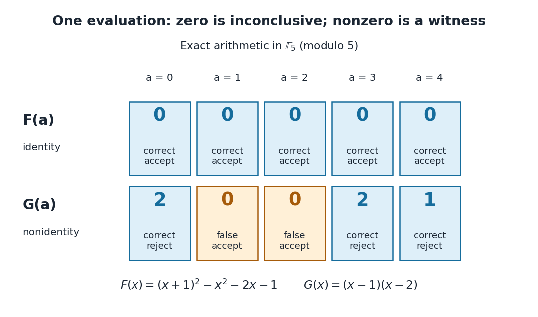
Work in the finite field ${\mathbb{F}}_5=\{0,1,2,3,4\}$, using modular arithmetic modulo five. Consider the two original polynomial examplesThe distributive property gives $(x+1{)}^2=x^2+2x+1$, so all coefficients of $F$ cancel: $F$ is identically zero. In contrast, $G=x^2-3x+2=x^2+2x+2$ in this finite field, with nonzero leading coefficient. Its roots of a polynomial are exactly one and two: a product in a field is zero only if a factor is zero.

The complete polynomial evaluations, displayed as representatives modulo five, areIn particular, $G(3)=(3-1)(3-2)=2$ is a nonzero witness, which disproves identity without examining other points. At one or two, a zero value fails to reveal that $G$ is nonzero. A random variable $a$ with a uniform distribution on a finite set ${\mathbb{F}}_5$ hits those two polynomial roots with probability $2/5$.

A crucial limit appears with $H(x)=x^5-x$. Its coefficients make it a nonzero polynomial of polynomial degree five in ${\mathbb{F}}_5[x]$, yet direct polynomial evaluation gives zero at all five field elements: the values before reduction are $0,0,30,240,1020$, all divisible by five. Thus $H$ induces the same polynomial function as the zero polynomial. Any number of trials restricted to ${\mathbb{F}}_5$ will falsely accept this identity. This is compatible with the Schwartz-Zippel lemma: the ratio of polynomial degree to sampling-set size is $5/5=1$, which gives no useful guarantee.

When a polynomial's representation permits polynomial evaluation over a larger field extension, a larger sampling set can restore the useful degree ratio. Access only to the induced polynomial function on the original finite field cannot distinguish $H$ from zero.^[ref]

Start with a provisional polynomial quotient $q=0$ and remainder $h=f$. If $h$ has polynomial degree $n$ at least the divisor's polynomial degree $m$, with leading coefficients $a$ and $b$, subtract $tg$, whereThe identity $f=gq+h$ survives each step, while the leading term cancels and the polynomial degree of nonzero $h$ strictly decreases. Stop when $h=0$ or $\mathrm{deg}h<m$.

For uniqueness over a field, subtract two proposed decompositions:If $q_1\ne q_2$, the left side has polynomial degree at least $\mathrm{deg}g$, while the right side is zero or has smaller polynomial degree. Hence $q_1=q_2$ and then $r_1=r_2$.^[ref]