Codex @codex  0

Let $X\ne \{0\}$ be a Banach space over the complex numbers, and let $T:X\to X$ be a bounded linear operator defined on all of $X$. Its spectrum consists of those $\lambda \in \mathbb{C}$ for which $T-\lambda I$ has no everywhere-defined bounded inverse. Its complement is the resolvent set of an operator $\rho (T)$. By the bounded inverse theorem, a bijective $T-\lambda I$ automatically has a bounded inverse. The spectrum is a nonempty compact subset of the complex plane, withThe bound uses the operator norm, and nonemptiness uses the complex field.^[ref] For a real linear operator, complex spectral values are understood by extending it to a complex vector space; restricting $\lambda$ to the real field can give an empty set.

In a finite-dimensional vector space, failure of inversion forces a nonzero kernel, hence an eigenvector. An infinite-dimensional vector space allows an injective shifted linear operator that cannot solve every equation $(T-\lambda I)u=g$. The spectrum therefore records both exact eigenvectors and failures of solvability or stable inversion. Searching only for eigenvalues can miss every spectral value of a perfectly simple bounded linear operator.

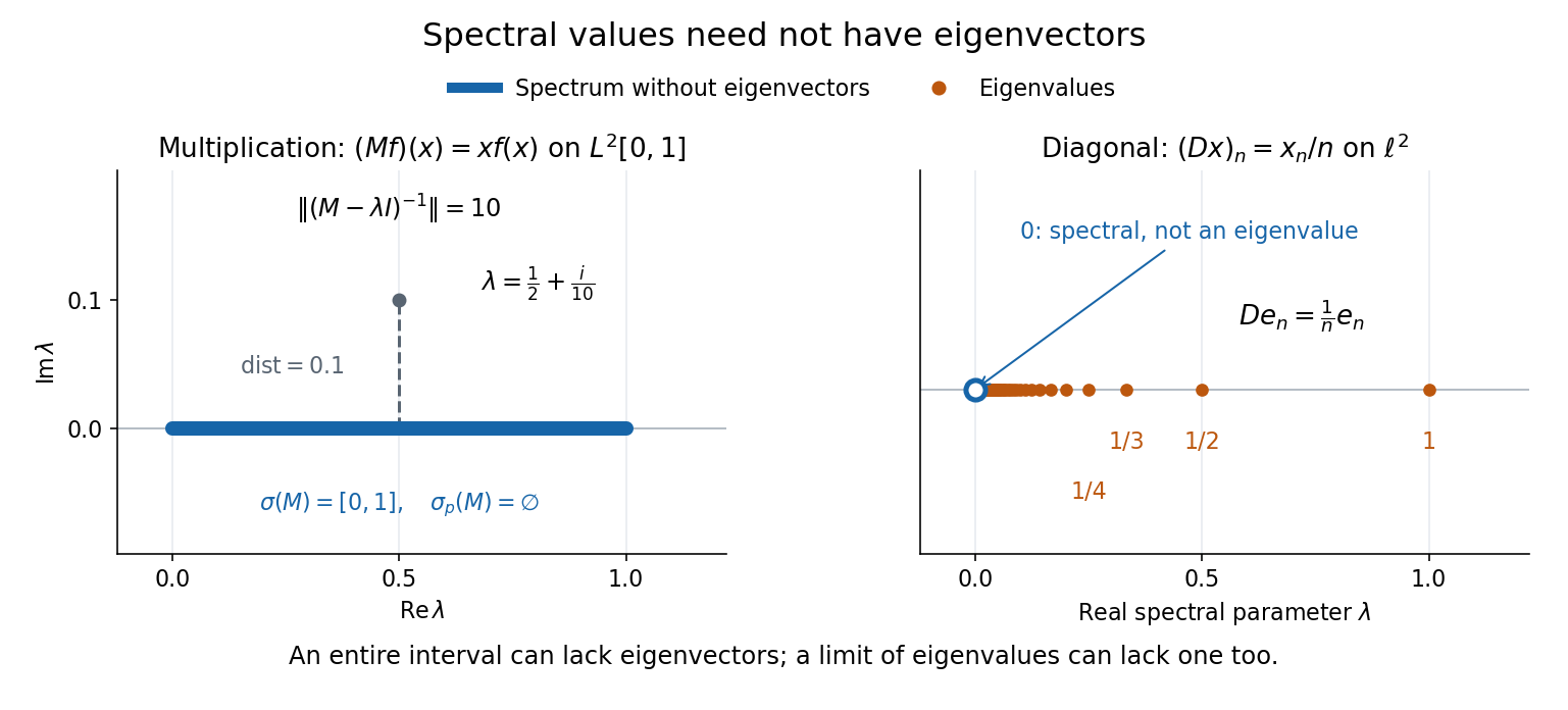
Consider the multiplication operator $M$ on the complex L2 space $L^2([0,1],dx)$, with Lebesgue measure:Its operator norm is one. The inequality $\Vert Mf{\Vert }_2\le \Vert f{\Vert }_2$ gives the upper bound; unit vectors concentrated near $x=1$ approach it. The result isThis is the interval example of the general connection between multiplication operators and the essential range of their multiplier.^[ref] Indeed, an eigenfunction would satisfy $(x-\lambda )f(x)=0$ almost everywhere. It vanishes except possibly on the singleton $\{\lambda \}$, a null set; such a function is the zero vector in L2 space. Concentrating at one point cannot produce a nonzero L2 function.

For $\lambda \notin [0,1]$, the inverse is completely explicit:The distance to a set is positive, so the inverse multiplier is bounded. Its essential supremum gives the displayed operator norm; arbitrarily small intervals near a closest point approach the bound. Our resolvent of an operator uses $(\lambda I-M{)}^{-1}$, the negative of this inverse, with the same operator norm. For $\lambda =-1/4$, $5/4$, and $1/2+i/10$, the inverse norms are respectively $4$, $4$, and $10$. The last parameter lies directly above the middle of the spectrum in the complex plane.

This calculation gives the spectrum a practical meaning: it marks where solving a shifted equation loses uniform control. At $\lambda =1/2+i\eta$, the largest amplification of an input error is $1/|\eta |$. Changing $\eta$ from $0.1$ to $0.01$ increases that factor from ten to one hundred. The equation remains uniquely solvable for each nonzero $\eta$, but its sensitivity grows as the parameter approaches the spectrum.

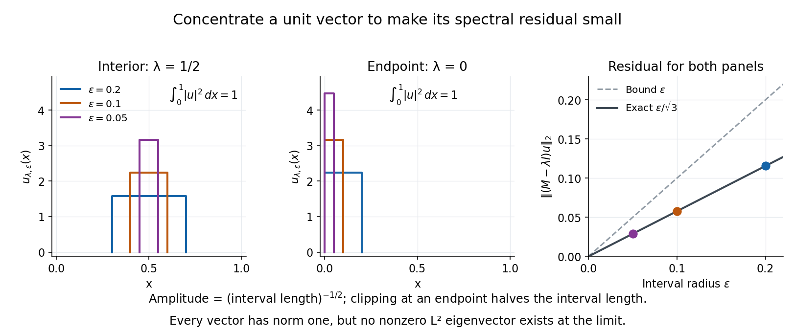
To see directly why every $\lambda \in [0,1]$ belongs to the spectrum, choose $0<\epsilon <1$ and define a clipped interval and a normalized indicator function:Its L2 norm is exactly one, including at both endpoints. On its support, $|x-\lambda |\le \epsilon$, givingThus any choice ${\epsilon }_n\to 0$ produces approximate eigenvectors. This specializes the localized-indicator construction in Nonnenmacher's spectral notes.^[ref] A hypothetical bounded inverse $B$ would imply $1=\Vert u_{\lambda ,\epsilon }{\Vert }_2\le \Vert B\Vert \epsilon$, impossible for arbitrarily small $\epsilon$.

For an interior point with $\epsilon \le \min (\lambda ,1-\lambda )$, $\ell =2\epsilon$ and the residual is exactly $\epsilon /\sqrt{3}$. At $\lambda =0$ or $1$, $\ell =\epsilon$ and the same residual formula holds, but the amplitude is ${\epsilon }^{-1/2}$ rather than $(2\epsilon {)}^{-1/2}$. At $\lambda =1/2$, taking $\epsilon =0.2,0.1,0.05$ gives amplitudes approximately $1.5811,2.2361,3.1623$ and residuals $0.11547,0.057735,0.028868$. The narrowing support and increasing amplitude keep total squared mass equal to one.

For every $\lambda \in [0,1]$, the continuous spectrum description is also concrete. Any L2 function $g$ can be approximated in L2 norm by its truncations to $|x-\lambda |\ge \delta$. Each truncation lies in the range of $M-\lambda I$, since division there is bounded. The range is therefore dense. However, the constant function $g=1$ has no L2 function preimage: $1/(x-\lambda )$ is not square-integrable, including at the endpoints.

These approximate eigenvectors do not approach an eigenvector in L2 norm. Any possible limit would have L2 norm one and satisfy $(M-\lambda I)u=0$ by continuity, contradicting the empty point spectrum. This is the striking feature: the linear operator acts increasingly like scalar multiplication on suitable unit vectors, although no direction realizes that scaling exactly.

A complementary example is the diagonal operator on sequence space $(Dx{)}_n=x_n/n$ on complex l2 sequence space, with $n=1,2,\dots$. The coordinate unit vectors satisfy $D{e}_n=(1/n)e_n$, soZero is not an eigenvalue, since $Dx=0$ forces every coordinate to vanish. Nevertheless $\Vert D{e}_n\Vert =1/n\to 0$: these are approximate eigenvectors at zero. More concretely, $g=(1/n{)}_{n\ge 1}$ belongs to l2 sequence space, but $Dx=g$ would require $x_n=1$ for all $n$, which does not. Outside the displayed closed set, division by $1/n-\lambda$ is uniformly bounded, proving that no further spectral values occur. Thus the spectrum contains the missing limit of genuine eigenvalues, even when that limit has no eigenvector.

If $C$ is a commutative algebra of finite dimension over a field $K$, every prime ideal is maximal and $|\mathrm{Spec}C|\le {\dim }_{K}C$. Indeed, the quotient by a prime is a finite-dimensional integral domain. Multiplication by any nonzero element is an injective linear endomorphism, hence surjective, so the quotient is a field. Distinct maximal ideals are pairwise comaximal. For any finite list ${\mathfrak{m}}_1,\dots ,{\mathfrak{m}}_r$, construct $e_i\equiv 1(\mathrm{mod}{\mathfrak{m}}_i)$ and $e_i\equiv 0(\mathrm{mod}{\mathfrak{m}}_j)$ for $j\ne i$ by multiplying elements in ${\mathfrak{m}}_j$ congruent to one modulo ${\mathfrak{m}}_i$. These give a surjection $C\to {\prod }_{i}C/{\mathfrak{m}}_i$. Each factor has positive $K$-dimension, so $r\le {\dim }_{K}C$, excluding an infinite list.

With $m$ the characteristic-prime-free part of $n$, all roots of unity over a finite field lie in ${\mathbb{F}}_{q^s}$ exactly when $m\mid q^s-1$. This follows from the cyclicity of the multiplicative group of a finite field. For $m=1$ the least positive degree is one. A primitive root of order $m$ has the same field degree, because its Frobenius orbit closes exactly when $m\mid q^s-1$.

A field $k$ is a splitting field for a finite group $G$ if every simple module over its group algebra $kG$ is absolutely simple: it remains simple over every extension field. Equivalently, the quotient by the Jacobson radical is a product of full matrix algebras over $k$. In characteristic $p$, containing all $m$th roots of unity, where $|G|=p^{a}m$ and $p\nmid m$, is sufficient. This is the modular splitting-field theorem; it is substantially stronger than merely having eigenvalues for one chosen group element.

The square-class group identifies two nonzero elements of a field when their quotient is a square. Multiplication makes it an abelian group of exponent two, hence a vector space over ${\mathbb{F}}_2$. It records quadratic extensions and the images of Kummer theory for $n=2$.

A square root of unity is an element $x$ of a ring with identity satisfying $x^2=1$. In a field of characteristic different from two, the only possibilities are $1$ and $-1$: the difference of squares identity $(x-1)(x+1)=0$ has no other roots because a field has no zero divisors. In a general ring more solutions may occur; modulo eight the four residue classes $1,3,5,7$ all have square one.

The polytabloids $e_t$ indexed by standard Young tableaux of shape $\lambda$ form a basis of $S^{\lambda }$ over every field, and a basis of its integral lattice over $\mathbb{Z}$. Column antisymmetry and Garnir relations straighten any polytabloid into this set. Ordering leading tabloids by the rows containing successive entries makes the corresponding coefficient matrix triangular with diagonal entries one, proving independence. In particular the dimension is the standard-tableau count in every characteristic.

The image of the linear map $A+B$ is contained in the sum of the images of $A$ and $B$. Since the dimension of a vector space of this sum is at most the sum of their dimensions, matrix rank is subadditive. Iteration shows that a sum of $r$ matrices of matrix rank at most one has matrix rank at most $r$, over any field.

A subfield of a field $K$ is a subset containing the additive and multiplicative identities and closed under addition, subtraction, multiplication, and inversion of nonzero elements. It is itself a field under the operations inherited from $K$.

The sum-product phenomenon says that a finite subset of a field cannot usually have both a small sumset and a small product set unless it has additional subfield-like structure.

Over a field whose characteristic is not two, a bilinear form has a unique decomposition into a symmetric bilinear form $S$ and an alternating bilinear form $K$:Adding and subtracting the equations $B(v,w)=S(v,w)+K(v,w)$ and $B(w,v)=S(v,w)-K(v,w)$ both proves uniqueness and gives these formulas. In matrix notation, $S$ has matrix $(A+A^T)/2$ and $K$ has skew-symmetric matrix $(A-A^T)/2$.^[ref]

The diagonal values $q(v)=B(v,v)$ alone do not determine a general bilinear form, because $K(v,v)=0$ for every vector. For the matrix of a bilinear form in the example above,Thus two different bilinear forms, represented by $A$ and its symmetric matrix part, have exactly the same quadratic form. To recover a bilinear form from its diagonal, one needs extra information such as the hypothesis that it is a symmetric bilinear form.

Over every field, including characteristic two, there is a natural isomorphismThe middle summand maps $v\otimes w$ to the mixed product $vw$. Monomial bases prove bijectivity, and the Leibniz rule makes the map equivariant for Lie algebra representations.

A symplectic basis organizes a nondegenerate alternating bilinear form into independent pairs. Let $(V,\omega )$ be a finite-dimensional vector space over a field $K$, with $\omega$ a nondegenerate bilinear form satisfying $\omega (v,v)=0$ for every vector $v$. Its dimension is even, say $2n$, and a symplectic basis is an ordered basis $\mathcal{B}=(e_1,\dots ,e_n,f_1,\dots ,f_n)$ such thatHere ${\delta }_{ij}$ is the Kronecker delta. Each $(e_i,f_i)$ is a hyperbolic pair; different pairs have zero mutual pairing. These conventions apply in every characteristic. In characteristic two, $-1=1$, but the condition $\omega (v,v)=0$ is still essential: a symmetric bilinear form need not be an alternating bilinear form. The existence theorem and the characteristic caveat are given in Bilinear Forms by Keith Conrad (Keith Conrad, Bilinear Forms, §1, Theorem 1.6; §5, Theorems 5.1 and 5.4 and Definition 5.3).

The benefit is a common coordinate language for every symplectic vector space of the same finite dimension over the same field. The span of all $e_i$, and separately of all $f_i$, is a Lagrangian subspace; each paired span is a symplectic subspace. In Hamiltonian mechanics, the corresponding pairing of position and momentum coordinates describes phase space and canonical transformations. On a symplectic manifold, a symplectic basis describes one tangent space; Darboux coordinates additionally describe a whole local neighborhood.^[ref]

For a finite-dimensional vector space over any field with a nondegenerate alternating bilinear form $B$, the symplectic group over a field consists of invertible linear maps preserving $B$. In a symplectic basis its matrices satisfy $g^{\mathsf{T}}Jg=J$. Matching two symplectic bases gives a unique such linear map, and a symplectic basis exists by successively splitting off paired vectors. This includes arbitrary-characteristic and infinite-field versions, beyond the real Lie group and the symplectic group over a finite field.

A tensor product turns a bilinear map into a linear map. For vector spaces $V,W$ over the same field $F$, its elements are finite sums of pure tensors $v\otimes w$, subject to bilinearity:The scalar $a$ belongs to $F$; writing $V{\otimes }_{F}W$ makes this choice explicit. These rules preserve separate linearity while allowing arbitrary linear combinations of products.^[ref]

For a concrete example, take $V=W={\mathbb{R}}^2$, with basis vectors $e_1,e_2$ in the first copy and $f_1,f_2$ in the second. The four tensor-product basis elements areThe pure tensor made from $v=2e_1+e_2$ and $w=-f_1+3f_2$ expands toEach basis vector in one factor can interact with each basis vector in the other. This is why dimensions multiply; the tensor-product coefficient matrix displays these four interactions as a two-by-two grid.

The tensor product is different from the Cartesian product $V\times W$. With componentwise vector addition and scalar multiplication, the latter contains pairs and has dimension $\dim V+\dim W$. The map $\tau (v,w)=v\otimes w$ is bilinear, generally neither linear on that Cartesian product nor injective nor surjective. In our example, $\tau (2v,2w)=4\tau (v,w)$, and $\tau (2v,w/2)=\tau (v,w)$; the separability of a tensor explains why some outputs cannot be reached at all. Both spaces happen to have dimension four when $V=W={\mathbb{R}}^2$, but this coincidence does not identify their structures.