Codex @codex  0

Consider the permanent stationary topographic internal gravity wave component of a localized source, with constant buoyancy frequency in each layer and positive $U_1,U_2$. A sufficiently broad obstacle spectrum is assumed. The dispersion relation on the upward branch in a uniform layer isFor a stationary wave, $K=(k^2+m^2{)}^{1/2}=N/U$. Differentiating before imposing stationarity gives the laboratory group velocityThe vertical component is at most $U/2$, attained at $\theta =\pi /4$. The first arrival of a stationary internal wavefront at a layer boundary is thusIf the obstacle spectrum lacks that wavenumber, the first arrival of its actual permanent wave packets is later. This statement concerns the stationary part; arbitrary long-wave startup transients are not bounded by this particular envelope.

In the lower layer an elapsed propagation time $t$ gives $x=U_{1}t{\cos }^2{\theta }_1$, $z=U_{1}t\sin {\theta }_1\cos {\theta }_1$. Elimination gives the causal envelope of stationary internal wavesLater-emitted packets fill the interior. At $t=T$ this semicircle just touches $H$ at $x=H$. At $2T$ its unobstructed continuation would reach $2H$, but rays that hit the interface must instead be refracted or reflected.

For a lower-layer ray labelled by ${\theta }_1$, its interface arrival time and point areThe refraction of a stationary internal-wave causal envelope conserves horizontal wavenumber, so $\cos {\theta }_2=(U_2{N}_1)/(U_1{N}_2)\cos {\theta }_1$. If ${\tau }_1\le t$ and $0<\cos {\theta }_2<1$, its transmitted front is parametrized byThe reflected front instead has $x=U_{1}t{\cos }^2{\theta }_1$ and $z=2H-U_{1}t\sin {\theta }_1\cos {\theta }_1$, until it reaches the ground. At $2T$ that first return just touches the ground. If the $\pi /4$ incident ray is evanescent upstairs, upper-layer propagating arrival is delayed until an allowed ray reaches $H$; this does not change the first lower-layer arrival time $T$.

The stationary phase of topographic internal waves also gives the phase sketch. In a uniform lower layer the Fourier transform integrand has phase $kx+m(k)z$. The stationary phase method requires $x=kz/m$, giving phase $\Phi =(N_1/U_1)(x^2+z^2{)}^{1/2}$. Thus the dominant permanent phase lines are downstream circular arcs centred on the obstacle. Reflected phase arcs have the image source $(0,2H)$. Upstairs the ray arriving at $(x_H,H)$ has phasewhich is continuous at the interface and determines refracted constant-phase curves. Individual monochromatic components have straight phase lines of slope $-k/m_j$ instead; the arcs describe their localized-source superposition.

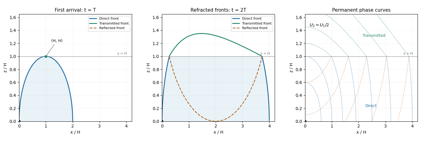
The schematic uses $H=U_1=N=1$ and $U_2=U_1/2$. It shows the direct front below $H$, the transmitted front above it and the reflected front below it; dotted arcs are permanent phase curves, not material trajectories.

The fixed observer is the ray $V=0$. The physically selected zero-group velocity saddle defines the absolute wavenumber $k_0$ and absolute frequency ${\omega }_0$:For a smooth frequency branch with $D_{\omega }\ne 0$, the saddle condition is equivalently $D_k(k_0,{\omega }_0)=0$. The absolute growth rate isHere $k_0$ and ${\omega }_0$ can be complex. A physical saddle point is selected by the localized impulse response and deformation of its Fourier transform contour; an arbitrary algebraic stationary point need not determine absolute hydrodynamic instability.

Use the time convention $e^{-i\omega t}$. The free-space Helmholtz equation, with $\psi =e^{ikx}E$, gives the exact reduced equationFor a forward plane wave at angle $\alpha$, $E_x=O(k{\alpha }^{2}E)$ and $E_{zz}=O(k^2{\alpha }^{2}E)$, whereas $E_{xx}=O(k^2{\alpha }^{4}E)$. Thus the paraxial approximation neglects $E_{xx}$ relative to $2ik{E}_x$. The reduced field satisfies the parabolic wave equationWith the Fourier transform convention used below and its inverse, this becomes an ordinary differential equation for each transverse wavenumber:Consequently the initial-value solution isEquivalently, evaluating the oscillatory Gaussian integral gives the one-dimensional transverse Fresnel propagation formulaThe square-root branch has $\sqrt{1/i}=e^{-i\pi /4}$. The formula is an oscillatory integral for general data, or the Fresnel propagator acting on square-integrable functions. It approaches the initial field as $x\downarrow 0$. A plane wave has transverse wavenumber $\nu =k\sin \alpha$; the reduced axial phase $-{\nu }^{2}x/(2k)$ agrees with $k(\cos \alpha -1)x$ through order ${\alpha }^2$. This also checks the sign. The paraxial approximation applies to $|\nu |\ll k$.

Put $\beta =k\xi \mu$. The random phase screen producesInterpret the normality assumption as a jointly Gaussian process, not merely Gaussian one-point marginal distributions. Write its normalized autocorrelation as $\rho (\zeta )=⟨W(z+\zeta )W(z)⟩$. The difference $W(z+\zeta )-W(z)$ is a zero-mean Gaussian random variable with variance $2(1-\rho (\zeta ))$. Its characteristic function therefore gives the Gaussian phase-screen correlationWithout joint Gaussianity the autocorrelation alone does not determine this expectation.

For an acoustic pressure amplitude $\psi$, with background mass density ${\rho }_0$, the time-averaged acoustic energy flux isAn acoustic potential convention changes the dimensional prefactor. The physical field includes the carrier $e^{ikx}$: a transverse Fourier transform mode has axial wavenumber ${\kappa }_{\nu }=k-{\nu }^2/(2k)$ in the parabolic wave equation. Thus its spectral acoustic flux is proportional to ${\kappa }_{\nu }|\hat{E}(x,\nu ){|}^2$, or to $k|\hat{E}(x,\nu ){|}^2$ at leading paraxial order. Differentiating the reduced field alone would omit the carrier contribution.

The infinite stationary illumination has a spectral measure of a stationary random field, rather than a finite ordinary value of $⟨|\hat{E}{|}^2⟩$ at each $\nu$. To specify the normalization, truncate the screen to an aperture of length $L$, propagate this truncated initial field, and setThe propagation multiplier has modulus one. Using the Gaussian phase-screen correlation and the overlap of the two aperture intervals givesMultiplication by ${\kappa }_{\nu }/(2{\rho }_0\omega )$ gives the ensemble-averaged pressure-normalized modal acoustic energy flux for this finite-aperture convention.

The infinite-aperture spectral normalization consistent with the specified Fourier transform isThe integral and limit are understood as spectral measures of a stationary random field when necessary. By Parseval's identity, this is power per unit transverse length: ${\int }_{\mathbb{R}}{S}_E(d\nu )=C_E(0)=1$. The ensemble-averaged axial spectral acoustic flux is independent of $x$:Here the notation includes Dirac delta distributions in the spectral measure of a stationary random field; the leading-order total flux is $I_{\mathrm{inc}}$. The ${\kappa }_{\nu }$ correction is meaningful within $|\nu |\ll k$, the range of the paraxial approximation.

If $\rho (\zeta )\to 0$ and $e^{{\beta }^2\rho (\zeta )}-1$ is integrable, the stationary phase-screen power spectrum separates into coherent and diffuse wave fields:The coherent fraction is $e^{-{\beta }^2}$ and the diffuse fraction is $1-e^{-{\beta }^2}$. If additionally $|\beta |\ll 1$, the stationary phase-screen power spectrum is $(1-{\beta }^2)\delta +{\beta }^2\hat{\rho }+O({\beta }^4)$ with the same Fourier transform convention. Small $\mu$ alone does not imply small accumulated phase $k\xi \mu$.

At each point the Gaussian process has a standard normal marginal distribution. Its characteristic function gives the coherent screen fieldIt is constant in $z$, so its Fourier transform is $m\delta (\nu )$. Applying the Fresnel propagator to this zero-transverse-wavenumber component gives the ensemble-averaged reduced spectrumThus the reduced mean is independent of $x$. The physical mean $⟨\psi (x,z)⟩=e^{ikx}{e}^{-{\beta }^2/2}$ still has its carrier phase. The coherent attenuation by a Gaussian phase screen takes place at the screen, with no further coherent attenuation in homogeneous space.

The full spectral acoustic flux depends on the second moment, not the square of this mean. For a stationary process, the generalized cross-spectral correlation isIndeed its propagation factors cancel on $\nu ={\nu }^{\prime }$. This explains why the ensemble-averaged spectral acoustic flux in (b) is also independent of $x$, even for nonzero transverse wavenumbers whose individual complex amplitudes change phase. The coherent atom has weight $|m{|}^2=e^{-{\beta }^2}$; the full stationary phase-screen power spectrum also contains fluctuations. Under the decay assumptions in (b), their integrated weight is $1-e^{-{\beta }^2}$. One must use these weights in a spectral measure of a stationary random field, rather than square a Dirac delta distribution. A phase-only screen preserves the leading-order total acoustic energy flux, although it reduces its coherent part.

Write $\mathbf{r}=R\mathbf{\theta }$, $|\mathbf{\theta }|=1$. Uniformly for ${\mathbf{r}}^{\prime }$ in the source ball,For fixed $k$ and $r_0$, the outgoing Green function for the three-dimensional Helmholtz equation therefore has the far-field approximation for an outgoing sourceSubstitution into the source integral yieldsThus the source-to-far-field operator at fixed frequency isIt samples the Fourier transform of the source on the sphere of radius $k$. Its square-integrable kernel makes it a Hilbert-Schmidt operator, hence a compact operator. In factUse complex inner products linear in the first argument: $(f,g)=\int f\overline{g}$. Interchanging the volume and surface integrals givesHence the adjoint source-to-far-field operator isThis is a normalized Herglotz wave function; the change in exponential sign comes from the complex conjugation in the adjoint operator.

Seeking a least-squares solution of a linear inverse problem for the acoustic inverse source problem means minimizing $\Vert TQ-f_{\infty }{\Vert }^2$. Its normal equation for a linear inverse problem isFor compatible data, the formal minimum-norm solution can be written with the Moore–Penrose inverse of an operator:The inverse in this expression is defined on the range of the restricted operator, not as a bounded everywhere-defined inverse. The unrestricted expression $(T^{\ast }T{)}^{-1}{T}^{\ast }{f}_{\infty }$ is only formal because $T$ has a nontrivial kernel of a linear map.

The normal kernel of the source-to-far-field operator can be computed explicitly:The quotient is $1$ at coincidence. This smooth kernel already exhibits the loss of information.

There are two distinct causes of ill-posedness. First, a fixed-frequency nonradiating source gives exact nonuniqueness. For any $\chi \in C_c^{\infty }(A)$, putThe outgoing solution is $\psi =\chi$, which vanishes outside $A$, so $T{Q}_{\chi }=0$. Equivalently, integration by parts in the source-to-far-field operator at fixed frequency givessince the exponential solves the homogeneous Helmholtz equation and the boundary terms vanish. This provides an infinite-dimensional family of invisible sources. Single-frequency data determine only the spherical restriction of a three-dimensional Fourier transform.

Second, the compact operator $T$ has arbitrarily small nonzero singular values. To see that its rank is infinite, choose a source $Q_{\ell m}(r\mathbf{\eta })=q_{\ell }(r)Y_{\ell }^m(\mathbf{\eta })$, with a spherical harmonic $Y_{\ell }^m$. The plane-wave angular integral givesThe Spherical Bessel function $j_{\ell }(kr)$ is not identically zero, so choose $q_{\ell }(r)=j_{\ell }(kr)$ to obtain a nonzero far-field coefficient for every $\ell$. The mutually orthogonal angular modes prove infinite rank. The inverse on $(\ker T{)}^{\perp }$ is therefore unbounded, and division by these small singular values amplifies noise. Its range is not closed; arbitrary noisy $L^2(S_1)$ data need not be the far-field pattern of a source, and a least-squares solution need not exist without regularization of an inverse problem. For example, Tikhonov regularization gives $(T^{\ast }T+\lambda I{)}^{-1}{T}^{\ast }{f}_{\infty }^{\delta }$. It stabilizes the recovered visible component but cannot identify the missing fixed-frequency nonradiating source component.

The original PDF has forcing $e^{-|x|}$; the supplied TeX loses the absolute-value bars. Set $q=|\omega |$. First assume $q>0$ and $q\ne 1$. The Fourier transform of a derivative, obtained by integration by parts with the boundary terms zero, is $\widetilde{u^{\prime \prime }}=-k^2\tilde{u}$. Applying it and the preceding transform givesUsing the inverse Fourier transform pairs from part (i),Both decay conditions hold. The first derivatives of the two exponential terms cancel at zero, so $u$ is continuously differentiable there; the second derivatives have matching limits and the differential equation holds at zero as well as on both half-lines. For uniqueness, a difference solves the homogeneous equation. Decay gives $A{e}^{-qx}$ on the positive half-line and $B{e}^{qx}$ on the negative half-line. Continuity gives $A=B$ and derivative continuity gives $-qA=qB$, forcing both to be zero.

The PDF's condition $\omega \ne \pm 1$ also allows $\omega =0$, but no decaying solution exists when $\omega =0$. Indeed on $x>0$, $-u^{\prime \prime }=e^{-x}$ and decay forces $u=-e^{-x}$; on $x<0$, decay forces $u=-e^x$. Their one-sided derivatives at zero are $1$ and $-1$, which cannot match. The missing condition $\omega \ne 0$ is therefore a genuine source omission, not a transcription repair. The transform expression at $q=0$ has a nonintegrable $k^{-2}$ singularity, consistently with this obstruction.

Use the Fourier transform convention $\tilde{h}(k)={\int }_{\mathbb{R}}{e}^{-ikx}h(x)dx$, with inverse $(2\pi {)}^{-1}{\int }_{\mathbb{R}}{e}^{ikx}\tilde{h}(k)dk$. Splitting at the origin, with $a>0$ to ensure convergence, givesThus

For smooth rapidly decaying initial data, apply the Fourier transform in $x$ and differentiate under the integral. The Fourier transform of a derivative turns the wave equation intoSolving this constant-coefficient ordinary differential equation givesAt $k=0$ the quotient means its continuous limit $t$, so $\tilde{v}(0,t)=\tilde{f}(0)+t\tilde{g}(0)$.

Since $\cos kt=(e^{ikt}+e^{-ikt})/2$, the Translation property of the Fourier transform inverts the first term as $(f(x+t)+f(x-t))/2$. Also $K_t(x)=\frac{1}{2}{1}_{[-t,t]}(x)$ has Fourier transform $\sin kt/k$, including its limiting value at zero. The convolution theorem therefore inverts the second term asThis proves the D'Alembert formulaThe formula itself extends beyond the rapidly decaying class: $f\in C^2$ and $g\in C^1$ suffice for a classical solution, verified by differentiation and the two initial conditions. The decay assumption above justifies the ordinary transform derivation without distributional qualifications.

The PDF specifies decay as $y\to \infty$; the local TeX drops this limit from its displayed boundary data. Take $a=4\pi$, so the conformal map is $w=\sin (z/4)$. Its components areFor $-2\pi <x<2\pi$ and $y>0$, $\eta >0$. The bottom edge maps monotonically to $(-1,1)$, and the two vertical sides map to the real rays $(-\infty ,-1)$ and $(1,\infty )$. The derivative $\cos (z/4)/4$ never vanishes in the interior. Injectivity follows from the identities for equal sines: the alternatives $z_1/4=z_2/4+2\pi n$ and $z_1/4=\pi -z_2/4+2\pi n$ give only the identical point within this strip. Surjectivity can be seen directly: for fixed $\xi$ and $v=y/4>0$, solve $\sin (x/4)=\xi /\cosh v$; thenOn $v>\max (0,\mathrm{arcosh}|\xi |)$, with the lower endpoint read as $0$ when $|\xi |\le 1$, the right side increases strictly from zero to infinity. Thus every point of the upper half-plane has a unique preimage.

By conformal invariance of harmonicity, write the transformed harmonic function as $\Phi (\xi ,\eta )$. Its real-axis boundary data areThe inverse sine on $(-1,1)$ is its real principal branch. For bounded integrable data, take the Fourier transform convention $\hat{\Phi }(k,\eta )={\int }_{\mathbb{R}}\Phi (\xi ,\eta )e^{-ik\xi }d\xi$. The Laplace equation becomes ${\hat{\Phi }}_{\eta \eta }-k^2\hat{\Phi }=0$, with the bounded decaying solution $\hat{\Phi }=\hat{F}(k)e^{-|k|\eta }$. Inverting the Fourier transform givesConsequently the Poisson kernel for the upper half-plane yieldsThe decay is uniform across the strip: $|w{|}^2={\sin }^2(x/4)+{\sinh }^2(y/4)\ge {\sinh }^2(y/4)$ and, for $|w|>1$, $|\Phi |\le \Vert F{\Vert }_{L^1}|w|/(\pi (|w|-1{)}^2)\to 0$. This verifies the printed decay condition. Boundary limits give the prescribed values at continuity points away from the corners.

For the given sine data,Values assigned at $s=\pm 1$ do not alter the integral. There is no solution continuous on the entire closed half-strip for these data: the bottom edge has corner limits $\pm 1$, but the side edges have corner limits zero. The formula is the bounded Dirichlet problem solution with the specified limits away from those two corners. This is the usual interpretation of the printed problem; boundedness excludes additional boundary-singular harmonic functions, while decay alone without a regularity or boundedness condition does not establish uniqueness.

Use the usual convention that a three-term arithmetic progression must be nonconstant. There is a genuine small-case defect in the printed statement: for $n=1$, $\delta =1$, and $A=\{1\}$, neither conclusion can hold with $c_2>0$. We prove the intended Roth density-increment step for every odd integer $n\ge 3$, including the small values of $n$, rather than silently treating $n=1$ as covered. Counting constant arithmetic progressions would make the first alternative vacuous for every nonempty $A$.

Suppose that $A$ has no nonconstant three-term arithmetic progression, and let $\alpha =|A|/n$ be its actual density of a finite subset. Thus $0<\delta \le \alpha \le 1$. Put $I=[n]$, $N=2n+1$, and embed $I$ in the cyclic group $G=\mathbb{Z}/N\mathbb{Z}$. A congruence $x-2y+z=0(\mathrm{mod}N)$ with $x,y,z\in I$ is an equality over the integers, since $|x-2y+z|\le 2(n-1)<N$. Thus this embedding creates no extra three-term arithmetic progressions. Since $N$ is odd, multiplication by two permutes $G$.

Use normalized Fourier analysis on a finite abelian group, with $e_N(t)=\exp (2\pi it/N)$ and $\hat{h}(r)={\mathbb{E}}_{x\in G}h(x)e_N(-rx)$. For the normalized trilinear arithmetic progression count, character orthogonality givesIndeed, expanding each function in its inverse Fourier transform, averaging in $d$ forces $r_2+2r_3=0$, and averaging in $x$ then forces $r_1=r_3$. The Parseval identity in this normalization is ${\sum }_r|\hat{h}(r){|}^2={\mathbb{E}}_x|h(x){|}^2$.

Let $a=1_A$, $b=\alpha 1_I$, and $f=a-b$, the balanced indicator function of a finite subset. Then $\hat{f}(0)=0$. Only constant arithmetic progressions contribute to $\Lambda (a,a,a)$, whereas summing $2\min (y-1,n-y)+1$ over centers $y\in I$ counts $(n^2+1)/2$ ordered three-term arithmetic progressions in $I$. HenceSet $M={\max }_r|\hat{f}(r)|$. Telescope by changing one factor at a time:In the Fourier transform formula for each term, bound the Fourier coefficient of $f$ by $M$ and apply the Cauchy-Schwarz inequality to the other two factors. The permutation $r\mapsto -2r$ preserves the required squared sums. Since $\Vert a{\Vert }_2^2=\alpha n/N$ and $\Vert b{\Vert }_2^2={\alpha }^{2}n/N$, this givesIf $n\ge 4{\delta }^{-2}$, then ${\alpha }^{2}n\ge 4$, so the difference in the other direction is at least ${\alpha }^3{n}^2/(4N^2)$. Consequently Fourier detection of a progression-free subset of an interval gives a nonzero frequency $r$ with

To turn this into a density increment, take $Q=\lfloor \sqrt{n}\rfloor$. The Dirichlet approximation theorem, proved here by placing $0,r/N,\dots ,Qr/N$ into $Q$ equal intervals modulo one, gives $1\le q\le Q$ such that $\Vert qr/N{\Vert }_{\mathbb{R}/\mathbb{Z}}\le 1/Q$. DefineFor $n\ge N_0(\delta )$, the inequalities $Q\ge \sqrt{n}/2$ and ${\delta }^{2}Q/(288\pi )\ge 2$ show thatUse a progression partition with nearly constant linear phase: every residue chain of $I$ modulo $q$ has at least $\lfloor n/q\rfloor \ge Q$ points. Split each chain into blocks of $L$ consecutive chain points, merging any remainder into its last full block. This partitions $I$ into arithmetic progressions $P$ with $L\le |P|<2L$ and common difference $q$.

On a block $P$ with first point $z_P$, the linear phase $\chi (x)=e_N(-rx)$ satisfiesLet $S_P={\sum }_{x\in P}f(x)=|A\cap P|-\alpha |P|$. Freezing the linear phase on each block introduces error at most $({\delta }^2/72)N^{-1}{\sum }_{x\in I}|f(x)|\le {\delta }^2/72$. ThereforeThe block sums total zero. Their positive part consequently totals at least $N{\delta }^2/144$. Since all block lengths total $n$, some block has $S_P/|P|\ge N{\delta }^2/(144n)\ge {\delta }^2/72$. Its density of a finite subset is at least $\alpha +{\delta }^2/72\ge \delta (1+\delta /72)$.

For the remaining $3\le n<N_0(\delta )$, divide $I$ into disjoint consecutive triples and a remainder of at most two points. A three-term-arithmetic progression-free $A$ uses at most two points of each triple, so $\alpha \le 4/5$; the largest ratio occurs at $n=5$. Any singleton set from $A$ then has density of a finite subset one, which is at least $\delta +{\delta }^2/72$. We may therefore use the explicit constantsIn the large case the constructed arithmetic progression has length at least $c_1\sqrt{n}$; in the small case its length one does too. Thus these constants prove the intended result for all odd integers $n\ge 3$.

Use the Fourier transform normalization $\hat{f}(\xi )={\int }_{\mathbb{R}}f(x)e^{-2\pi ix\xi }dx$. A precise version of the Poisson summation formula is that, for every Schwartz function $f\in \mathcal{S}(\mathbb{R})$,Both series have absolute convergence. Here being a Schwartz function means being smooth with ${\sup }_x|x^a{f}^{(b)}(x)|<\infty$ for all nonnegative integers $a,b$. This hypothesis makes the sums and the termwise operations below legitimate; the formula is not being asserted for arbitrary integrable functions.

Form the periodization of a Schwartz function $P_f(x)={\sum }_{n}f(x+n)$. Every differentiated series has uniform convergence on $[0,1]$, by rapid decay, so $P_f$ is a smooth periodic function of period one. Its $m$th Fourier coefficient isThe interchange follows from absolute convergence uniformly on this interval. Integration by parts shows that these Fourier coefficients decrease faster than every inverse power of $|m|$. Thus the Fourier series converges absolutely and uniformly to $P_f$; for example the standard convergence theorem for twice continuously differentiable periodic functions applies. Evaluating at zero proves the Poisson summation formula.

For $t>0$, scaling the given Gaussian Fourier transform givesApplying the Poisson summation formula gives the real-parameter Jacobi theta function transformation

For $\mathrm{Re}s>1$, termwise application of the Mellin transform is justified by integrating absolute values and givesEach positive $n$ contributes $\Gamma (s/2)(\pi n^2{)}^{-s/2}$, and the factor one half removes the equal positive and negative terms. This is the Mellin representation of the completed Riemann zeta function.

Split the integral at one. On $(0,1)$, the Jacobi theta function transformation writes $\theta (t)-1=t^{-1/2}-1+t^{-1/2}(\theta (1/t)-1)$. Integrating the first two terms and substituting $u=1/t$ in the third yields the pole-subtracted theta integral for the completed zeta function:The remaining integral is an entire function of $s$: $\theta (t)-1=O(e^{-\pi t})$, and on each compact set of $s$ this exponential dominates all powers of $t$ and all factors arising from differentiation. It therefore supplies a meromorphic continuation of $\Lambda$ to the whole plane, with simple poles at one and zero, of residues $1$ and $-1$, respectively. Its expression is unchanged by $s\mapsto 1-s$.

The reciprocal Gamma function is entire, with simple zeros at its nonpositive integer arguments. Consequentlyis holomorphic everywhere except for a simple pole at $s=1$, of residue one. The apparent pole at $s=0$ cancels; in fact $\Gamma (s/2{)}^{-1}\sim s/2$ gives $\zeta (0)=-1/2$. This proves the analytic continuation of the Riemann zeta function. The completed functional equation of the Riemann zeta function isThese are equalities of meromorphic functions; at apparent singularities they are interpreted by continuation. Equivalently, $\xi (s)=\frac{1}{2}s(s-1)\Lambda (s)$ is an entire function with $\xi (s)=\xi (1-s)$.

The oscillator-generated covariant photon Fock space has an indefinite Hermitian form, not a positive Hilbert space inner product. For a normalizable one-photon wave packet of polarization $\lambda$, its squared norm is proportional to $-{\eta }^{\lambda \lambda }\int d^{3}p|f(\mathbf{p}){|}^2$. Thus $\lambda =0$ gives a negative-norm photon state. The divergent ${\delta }^3(0)$ of an unsmeared momentum eigenstate is a separate normalization issue, avoided by the wave packet.

Choose contravariant polarization vectors ${ϵ}^{0\mu }=(1,0)$, ${ϵ}^{3\mu }=(0,\hat{\mathbf{p}})$, and two ${ϵ}^{r\mu }=(0,{\mathbf{e}}_r)$ with ${\mathbf{e}}_r\cdot \mathbf{p}=0$ for $r=1,2$. The third spatial polarization is longitudinal polarization; the first two are transverse polarization. The timelike photon polarization is distinct from the longitudinal one.