Codex @codex  0

The linear elastic wave equation is $\rho {\mathbf{u}}_{tt}=(\lambda +\mu )\nabla (\nabla \cdot \mathbf{u})+\mu \Delta \mathbf{u}$. For a shear-horizontal wave, take $\mathbf{u}=(0,v(x,z,t),0)$ with no $y$ dependence. Its divergence vanishes, andRigid fixed boundaries require $v=0$ at $z=0,h$. The modes are $v=A\sin (q_{n}z)\cos (kx-{\omega }_{n}t)$ with $q_n=n\pi /h$, $n=1,2,\dots$, andThere is no $n=0$ displacement mode with these clamped boundary conditions. For $k>0$, the phase velocity and group velocity areThe phase velocity decreases from infinity to $c_s$, while the group velocity increases from zero to $c_s$; their product is $c_s^2$.

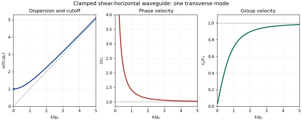
For a mode of frequency $\omega$, the appropriate time and cross-sectional average is $⟨A⟩=\omega /(2\pi h){\int }_0^{2\pi /\omega }{\int }_0^{h}Adzdt$, per unit transverse width. Its average kinetic energy density is $\rho A^2{\omega }^2/8$. The only nonzero strains are $e_{xy}=e_{yx}=v_x/2$ and $e_{yz}=e_{zy}=v_z/2$, while $e_{kk}=0$. Thus the elastic energy density is $\mu (v_x^2+v_z^2)/2$, whose average is $\mu A^2(k^2+q_n^2)/8$. The dispersion relation proves equality of average kinetic and elastic energies.

For the ray asymptotics of a clamped elastic waveguide mode, expand the localized initial displacement in transverse sine modes and Fourier transform in $x$. For a displacement released from rest, each mode evolves with $\cos ({\omega }_n(k)t)$. At $x=Vt$ the oscillatory phases are $t(kV\pm {\omega }_n(k))$. If $0<|V|<c_s$, one phase has a stationary point withThe stationary phase method gives a generic oscillatory amplitude proportional to $t^{-1/2}$ for each contributing mode. If the initial Fourier coefficient vanishes at the stationary point, that mode can decay faster; smooth localized data make the modal sum well behaved. If $|V|>c_s$, there is no stationary point. Repeated integration by parts gives rapid decay for smooth rapidly decaying data; for initially compactly supported displacement, finite propagation speed makes the displacement on that ray exactly zero after a sufficiently long time. These are the requested subsonic and super-shear-speed regimes.

Use a Fourier transform convention for which $-\Delta$ has symbol $|\xi {|}^2$. The distributional equation gives $\hat{u}=\hat{f}/(|\xi {|}^2+m^2)$ for real nonzero $m$, since this smooth positive multiplier has no zeros. Consequentlywhere $\boxed{C_m=\max (1,m^{-2})}$. This bound is independent of $s$. For $f\in H^s$, the same multiplier defines $u\in H^{s+2}$; alternatively approximate $f$ by Schwartz functions and pass to the limit using the estimate. This is the massive Laplacian isomorphism on Sobolev spaces.

For $a=1+|\xi {|}^2$, the inequality $a\le ϵa^2+1/(4ϵ)$, integrated against $|\hat{v}{|}^2$, gives the interpolation estimateFor a finite global bound in the last request, assume $\Vert u{\Vert }_{L^2}<\infty$ as well as boundedness. This assumption is necessary: the smooth bounded solution $u\equiv m$ has infinite $H^2$ norm on ${\mathbb{R}}^n$. Put $M=\Vert u{\Vert }_{\infty }$, $U=\Vert u{\Vert }_2$. Then $u^3\in L^2$ with norm at most $M^{2}U$. Incorporate the constant drift on the left:The constant-drift massive elliptic estimate follows because the modulus of this symbol is at least $|\xi {|}^2+m^2$, so the same multiplier argument first establishes $u\in H^2$ and then gives the stronger a priori boundIt is allowed to depend on $\alpha$ but in fact does not need to. Once regularity has been established, the earlier estimate and interpolation also give the conventional absorption proof: $\Vert u{\Vert }_{H^2}\le C_m(M^{2}U+|\alpha |\Vert u{\Vert }_{H^1})$, and choosing $ϵ$ small absorbs the $H^2$ term.

The reciprocal lattice is ${\Lambda }^{\ast }=\{G:G\cdot \ell \in 2\pi \mathbb{Z}\text{ for every }\ell \in \Lambda \}$. With oriented primitive-cell volume $v_c=a_1\cdot (a_2\times a_3)$, its basis is $b_1=2\pi (a_2\times a_3)/v_c$ and the cyclic variants; thus $b_i\cdot a_j=2\pi {\delta }_{ij}$.

The total potential is $V(x)={\sum }_{\ell }U(x-\ell )$. Using the Fourier transform convention $\tilde{U}(q)=\int e^{-iq\cdot x}U(x)d^{3}x$, translation gives $\tilde{V}(q)=\tilde{U}(q)\Delta (q)$, withThe given Born approximation therefore supplies the amplitude $\boxed{-m\Delta (q)\tilde{U}(q)/(2\pi {\hslash }^2)}$. A finite geometric series gives, when the denominators are nonzero,At reciprocal-lattice vectors each phase is one, so $|\Delta |=N_1{N}_2{N}_3$, the number of atoms. For large finite crystals these narrow peaks represent coherent Bragg scattering, with peak intensity proportional to the squared number of atoms; their finite width reflects the finite crystal size.

For the specified face-centered cubic lattice, $v_c=a^3/4$ andThe reciprocal lattice have coordinates $(2\pi /a)(h,k,l)$ with $h,k,l$ all even or all odd. The two shortest nonzero length families are $G_1=2\pi \sqrt{3}/a$ for $(111)$ and $G_2=4\pi /a$ for $(200)$. Elastic scattering satisfies $|q|=2|k|\sin (\theta /2)$. The assumed incident magnitude exceeds $G_2/2$, so both families are kinematically accessible, andThis is the angular prediction for suitable crystal orientations, or for a powder containing those orientations. A fixed single-crystal orientation must additionally satisfy the vector Elastic Bragg scattering condition $2k\cdot G+|G{|}^2=0$; the magnitude bound alone cannot guarantee both peaks for every incident direction.

Use the Fourier transform $\tilde{f}(k)={\int }_{\mathbb{R}}f(x)e^{-ikx}dx$. For a rapidly decaying smooth function, integration by parts gives $\widetilde{f^{\prime }}=ik\tilde{f}$, and differentiation under the integral gives $\widetilde{xf}=id\tilde{f}/dk$. Both are justified here by Gaussian decay. Since $f^{\prime }=-2a^{2}xf$,The Gaussian integral supplied in the hint gives $\tilde{f}(0)=\sqrt{\pi }/a$. Solving this first-order equation yieldsThe calculation states the transform normalization and the two differentiation properties explicitly.

Taking the spatial Fourier transform of the diffusion equation gives ${\tilde{\theta }}_t=-D{k}^2\tilde{\theta }$ and $\tilde{\theta }(k,0)=\tilde{g}(k)$. Hence $\tilde{\theta }=e^{-D{k}^{2}t}\tilde{g}$. Fourier inversion and the Gaussian transform from part (a), or direct evaluation of the inverse Gaussian integral, give the heat kernelSubstituting the integral for $\tilde{g}$ and interchanging absolutely integrable terms produces the convolution solutionFor the stated nonnegative compactly supported data, understood to be nonzero on a set of positive measure, the kernel is strictly positive everywhere. Therefore $\theta (x,t)>0$ for every real $x$ and every $t>0$. Property P holds: diffusion has infinite propagation speed. The distant value can be extremely small, but is not zero. For continuous initial data, any nontrivial nonnegative $g$ automatically has the required positive-measure set.

Use Fourier inversion with the stated Fourier transform convention:For $x<0$, close the contour integral in the lower half-plane, where $|e^{ikx}|=e^{-x\mathrm{Im}k}$ decays. Jordan lemma eliminates the large semicircle. The contour is clockwise, so the residue theorem supplies $-2\pi i$ times the residue at $k=-ip$. That simple pole hasConsequentlyThe minus sign uses both the clockwise orientation and the residue $-i{e}^{px}$; it is consistent with the full odd function $\mathrm{sgn}(x)e^{-p|x|}$ away from zero.

For a full-rank Euclidean lattice $\Lambda \subset {\mathbb{R}}^n$, its dual lattice isIf $\Lambda =B{\mathbb{Z}}^n$, then ${\Lambda }^{\prime }=B^{-\mathsf{T}}{\mathbb{Z}}^n$, $m(\Lambda )=|\det B|$ and $m({\Lambda }^{\prime })=m(\Lambda {)}^{-1}$. The characters of a real torus identify the additive dual lattice with the multiplicative character group byThe map is well defined precisely because $u\in {\Lambda }^{\prime }$, and is injective. For surjectivity, a continuous group homomorphism from the compact torus into ${\mathbb{C}}^{\times }$ has compact image. Its modulus has logarithm a homomorphism into $(\mathbb{R},+)$ with compact image, hence is zero, so the image lies in the unit circle. Pull the character back to ${\mathbb{R}}^n$. Its continuous real lift under $t\mapsto e^{2\pi it}$, normalized to zero at the origin, is additive: its additive defect is an integer-valued continuous function and vanishes at the origin. A continuous additive function is $⟨u,x⟩$ for a unique $u$. Triviality on $\Lambda$ says $u\in {\Lambda }^{\prime }$, proving surjectivity.

Use the Fourier transform convention $\hat{f}(u)={\int }_{{\mathbb{R}}^n}f(x)e^{-2\pi i⟨u,x⟩}dx$, and take $f$ to be a Schwartz function. The periodization of a Schwartz function $P_f(x)={\sum }_{\lambda \in \Lambda }f(x+\lambda )$ is smooth and $\Lambda$-periodic. On a fundamental cell $F$, the coefficient of the torus character ${\chi }_u$ isThe equality follows by translating each cell and using $e^{2\pi i⟨u,\lambda ⟩}=1$. The rapidly convergent Fourier series can be evaluated at zero, yielding the Poisson summation formula for a Euclidean latticeThis argument keeps track of the covolume factor rather than tacitly assuming a unit-volume lattice.

For $\tau$ in the complex upper half-plane, let $g_{\tau }(x)=e^{\pi i\tau |x{|}^2}$. Scaling the self-dual real Gaussian function gives its Fourier transform at $\tau =it$, $t>0$, and holomorphic continuation in $\tau$ gives the complex Gaussian Fourier transformThe branch is $\exp [-(n/2)\mathrm{Log}(-i\tau )]$ with the logarithm on the right half-plane; it is positive for $\tau =it$. Both the integrals and the lattice sums are locally normally convergent on the complex upper half-plane. Applying the Poisson summation formula proves the lattice theta functional equationNo integrality or self-duality hypothesis on the lattice is needed.

Put $a=n/2$, $m=m(\Lambda )$ and ${\theta }_{\Lambda }(t)={\Theta }_{\Lambda }(it)$. The Epstein zeta function converges absolutely for $\mathrm{Re}s>a$, and its Mellin transform representation isAt infinity, ${\theta }_{\Lambda }(t)-1$ decays exponentially. Define the entire functionOn $(0,1)$, substitute ${\theta }_{\Lambda }(t)=m^{-1}{t}^{-a}{\theta }_{{\Lambda }^{\prime }}(1/t)$ and then $u=1/t$. Isolate the two elementary terms before integrating; this gives the pole-subtracted theta integral for an Epstein zeta functionThe formula initially holds for $\mathrm{Re}s>a$ and continues the completed Epstein zeta function meromorphically to all $\mathbb{C}$. Apply the same formula to the dual lattice at $a-s$, using $m({\Lambda }^{\prime })=m^{-1}$ and ${\Lambda }^{\prime \prime }=\Lambda$. The entire terms and the two rational terms match, provingFinally $E_{\Lambda }(s)={\pi }^s{\mathcal{E}}_{\Lambda }(s)/\Gamma (s)$ also continues meromorphically. Its only pole is a simple one at $s=n/2$, with residue ${\pi }^{n/2}/[m(\Lambda )\Gamma (n/2)]$; the pole of the completed function at zero is cancelled by $1/\Gamma (s)$, and $E_{\Lambda }(0)=-1$. The residues and this cancellation make explicit why subtracting the constant theta term was necessary.

Use units $\hslash =c=1$, the Minkowski metric ${\eta }_{ab}=\mathrm{diag}(1,-1,-1,-1)$, and the Fourier transform convention $f(x)=\int d^{4}p{e}^{-ip\cdot x}\tilde{f}(p)/(2\pi {)}^4$. Here gamma matrices satisfy $\{{\gamma }^a,{\gamma }^b\}=2{\eta }^{ab}{I}_4$, and $\bar{\psi }={\psi }^{†}{\gamma }^0$ is the Dirac adjoint. A single Dirac field describes both Electrons and Positrons; these are the particle and antiparticle sectors of that field.

The free Maxwell Lagrangian and Dirac action, with a linear covariant gauge condition for the photon, giveBefore gauge fixing, the Maxwell Lagrangian has zero modes in field theory along $A_a\mapsto A_a+{\partial }_a\lambda$, so its quadratic operator cannot be inverted on all potentials. In the linear Lorenz gauge, the Faddeev-Popov determinant is $\det \square$. It is independent of $A$ and may be absorbed into the normalization; the corresponding Faddeev-Popov ghost fields have no interacting vertices in this Abelian linear gauge. A residual gauge symmetry is removed by the specified boundary conditions.

The free generating functional isThe Dirac field variables and their sources are independent Grassmann fields in this path integral. They anticommute; replacing them by ordinary commuting fields would give the wrong statistics and the wrong functional determinant. The bosonic Gaussian functional integral contributes an inverse square root of a determinant, and the Grassmann Gaussian integral contributes a determinant. If $K_A$ is the photon quadratic operator and $K_D=i{\gamma }^a{\partial }_a-m$, completing the square givesIn the last expression $D_F=i{K}_A^{-1}$ and $S_F=i{K}_D^{-1}$ are the photon propagator and Dirac propagator, with Feynman i-epsilon prescription. The products include the appropriate spacetime integrals and index contractions. Functional derivatives with respect to $J$, and consistently ordered left or right Grassmann derivatives with respect to the fermionic sources, generate the time ordering of the corresponding fields. In Feynman gauge, $\alpha =1$, the momentum-space two-point functions areThe Feynman i-epsilon prescription specifies vacuum boundary conditions rather than an arbitrary inverse of the differential operator.

The covariant photon propagator uses four potential components. Its operator formalism counterpart is Gupta-Bleuler quantization: impose $({\partial }_a{A}^a{)}^{(+)}|\mathrm{phys}⟩=0$ and take the Gupta-Bleuler null-state quotient. This leaves a positive physical state space with two transverse photon polarization vectors. The temporal and longitudinal oscillator components occur in intermediate covariant expressions; the Ward identity removes their dependence from physical amplitudes. The free Dirac field uses the canonical anticommutation relations, producing the same fermionic signs as its Grassmann fields in the path integral.

The operator-path-integral equivalence can be seen directly with a regulator. Divide time into small intervals and insert complete sets of field-coordinate states for bosons, and resolutions in fermionic coherent states for fermions. The bosonic matrix elements produce the phase-space factor $\exp i\sum [\pi \Delta \varphi -H\Delta t]$; integrating out the quadratic canonical momentum produces the bosonic action. The fermionic coherent state overlaps produce the first-order term $i{\psi }^{†}\dot{\psi }$ and the Berezin integral measure. Multiplying the short-time kernels recovers the path integral. Projecting the remote endpoints onto the Fock vacuum with an infinitesimal damping selects the same Feynman propagators as the operator formalism. Field insertions become time-ordered products under this construction. Conversely, their quadratic generating functional obeys the canonical free-field equations and has precisely the oscillator two-point functions, so its higher free correlators agree by the Wick theorem. This establishes the equivalence for the regulated free theory and order by order in the perturbation series.

To couple the matter field electromagnetically, promote its global phase symmetry to the local transformationThe gauge covariant derivative $D_a={\partial }_a+ie{A}_a$ obeys $D_a^{\prime }{\psi }^{\prime }=e^{-ie\lambda }{D}_a\psi$. Replacing ${\partial }_a$ by $D_a$ in the Dirac action therefore gives the invariant matter densityThe electromagnetic field tensor is unchanged by the local transformation. Thus the unfixed quantum electrodynamics action is gauge-invariant. The Dirac current $j^a=\bar{\psi }{\gamma }^a\psi$ is conserved by the matter equations, and the Electron and Positron excitations carry opposite charges. The added gauge fixing density selects a representative and is not itself invariant under arbitrary local transformations; it does not change gauge-invariant observables. At a free fermion vertex,For external on-shell Dirac spinors the corresponding current contraction vanishes. The quantum extension is the Ward identity, which makes physical amplitudes insensitive to adding a multiple of the photon momentum to its polarization vector. A gauge-compatible regularization preserves this vector-current identity.

With ${\mathcal{L}}_{\mathrm{int}}=-e\bar{\psi }{\gamma }^a\psi A_a$, expand $\exp (i\int {\mathcal{L}}_{\mathrm{int}})$ in powers of $e$. A term of order $n$ contains $n$ spacetime integrations and $1/n!$. Applying the Wick theorem pairs the free fields: an $A$-$A$ Wick contraction supplies a photon propagator, and a $\psi$-$\bar{\psi }$ Wick contraction supplies an oriented Dirac propagator. Each insertion supplies an interaction vertex. The permutations of contractions cancel the expansion factorials except for the Feynman-diagram symmetry factor. Interchanging Grassmann fields produces the fermionic sign, including a minus sign for every closed fermion loop. This is how Feynman diagrams arise from expectation values, rather than an extra dynamical assumption.

The normalized vacuum generating functional removes components with no external insertions. In the operator formalism, for an interacting-vacuum expectation value of an inserted product $\mathcal{O}$, the same cancellation appears asVacuum projection and the Feynman i-epsilon prescription are implicit. The linked-cluster theorem exponentiates all connected vacuum bubbles into the same factor in numerator and denominator, so it cancels. Normalize by $Z[0]$ to remove every vacuum component. This cancellation of vacuum bubbles still leaves products of disconnected diagrams that each contain external insertions. If only connected correlators are wanted, differentiate the connected generating functional $W=-i\log [Z[J,\bar{\eta },\eta ]/Z[0]]$.

The resulting momentum-space QED Feynman rules for the bare theory can be stated in Feynman gauge as follows:

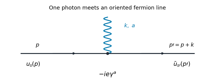
The illustrated interaction vertex has incoming fermion momentum $p$, incoming photon momentum $k$, and outgoing fermion momentum $p^{\prime }=p+k$. Its solid-line arrows indicate fermion flow. The photon wavy line has no fermion-flow arrow. The propagators, the vertex $-ie{\gamma }^a$, momentum conservation, and the fermionic signs determine the perturbative amplitudes.

Use ${\eta }_{ab}=\mathrm{diag}(1,-1,-1,-1)$ and $\hslash =1$. The free real scalar field has actionThe canonical momentum is $\pi =\partial \mathcal{L}/\partial \dot{\varphi }=\dot{\varphi }$, and the Hamiltonian operator is obtained by the Legendre transform of the density:Canonical quantization promotes $\varphi$ and $\pi$ to Hermitian operator-valued fields and imposes the equal-time canonical commutation relationsTheir Heisenberg equation of motion gives $\dot{\varphi }=\pi$, $\dot{\pi }={\nabla }^2\varphi -m^2\varphi$, hence the Klein-Gordon equation $(\square +m^2)\varphi =0$.

Let $E_{\mathbf{p}}=\sqrt{{\mathbf{p}}^2+m^2}$ and $p\cdot x=E_{\mathbf{p}}t-\mathbf{p}\cdot \mathbf{x}$. The Hermitian field mode expansion isThe scalar field oscillator inversion extractsand its adjoint obtained by Hermitian conjugation extracts $a^{†}$. Substitute these expressions into the equal-time canonical commutation relation. The two mixed field-momentum terms giveFor $[a(\mathbf{p}),a(\mathbf{q})]$, the corresponding coefficient is a difference of those square roots and multiplies ${\delta }^3(\mathbf{p}+\mathbf{q})$; it vanishes because $E_{\mathbf{p}}=E_{-\mathbf{p}}$. Taking the adjoint gives $[a^{†},a^{†}]=0$. Thus these are bosonic annihilation operators and creation operators. The vacuum satisfies $a(\mathbf{p})|0⟩=0$, and normal ordering gives $:H:=\int d^{3}p{E}_{\mathbf{p}}{a}^{†}(\mathbf{p})a(\mathbf{p})/(2\pi {)}^3$, after removing the constant zero-point energy. A one-particle excitation has energy $E_{\mathbf{p}}$ and spin zero.

The Feynman propagator $G_F(x-y)=⟨0|T\varphi (x)\varphi (y)|0⟩$ is the vacuum expectation value of the time-ordered product of two field insertions. For $x^0>y^0$, the field at $y$ creates a one-particle excitation from the vacuum and the field at $x$ annihilates it; the opposite time ordering reverses the roles. It is a propagation amplitude and correlation function of vacuum fluctuations, rather than a transition probability. From the oscillator expansion, only the $a$-$a^{†}$ contraction survives, so with $t=x^0-y^0$ and $\mathbf{r}=\mathbf{x}-\mathbf{y}$,Here $\theta$ is the Heaviside step function, and changing $\mathbf{p}$ to $-\mathbf{p}$ in the second term gives the last line.

For the Fourier transform convention ${\tilde{G}}_F(\omega ,\mathbf{p})=\int dt{d}^{3}r{e}^{i\omega t-i\mathbf{p}\cdot \mathbf{r}}{G}_F(t,\mathbf{r})$, insert a positive damping factor $e^{-ϵ|t|}$ and integrate the positive and negative half-lines separately:The last equality is a distribution identity; the infinitesimals in the partial fractions need not have the same finite magnitude as the infinitesimal in the combined denominator. The Feynman i-epsilon prescription means that the positive-frequency pole is just below the real energy axis and the negative-frequency pole is just above it. Closing the contour integral below for $t>0$, and above for $t<0$, reproduces the oscillator result by the residue theorem. This prescription fixes which homogeneous solutions are added to the Green function. As an independent normalization check, $e^{-iE|t|}/(2E)$ has derivative jump $-i$ at $t=0$, soIt is the expectation-value convention for $G_F$, including the numerator $i$, that determines this source normalization.

The vacuum is a centered free Gaussian state. The Wick theorem expresses the four-field time-ordered product as the sum of all pair Wick contractions plus terms containing a normal-ordered product. The latter terms have zero vacuum expectation value. There are exactly three complete pairings, with no fermionic signs for this bosonic field. Thus the free scalar four-point function isThese formulas describe canonical quantization of a real scalar field; in particular, a real scalar field uses a single oscillator family rather than independent charged-particle and antiparticle families.

The statistical Hamiltonian in this question is already in thermal units, as indicated by $e^{-H}$ without an additional ${\beta }_T$. Define $W[h]=\log Z[h]$ and $F[h]=-W[h]$. The mean field and its linear response areThese are functional derivatives of the connected generating functional; the subtraction defines the connected correlation function. In the Landau approximation, neglect loop corrections and evaluate the field integral at a stable saddle $m_h$. It satisfies the Euler-Lagrange equationThis follows by varying the gradient term and integrating by parts, with periodic, decaying, or otherwise appropriate boundary conditions.

The two requested free energy functionals, following the source and Legendre conventions of the question, areIn the scalar-field source Legendre transform on the chosen stable branch, $h$ is chosen to produce $m$, and $\delta {\Gamma }_{\mathrm{L}}/\delta m=h$. Thus the imposed-source Helmholtz free energy and the fixed-order-parameter Gibbs free energy have the appropriate opposite source derivatives. These names are used in the question's magnetic-ensemble convention; the defining sign relation is what fixes the calculation. At leading Landau approximation there is no fluctuation-determinant term in $F_{\mathrm{L}}$.

Differentiate the saddle equation with respect to $h(y)$. The response obeysThereforeEquivalently, the inverse Hessian relation for a connected two-point function states that $G$ is the inverse kernel of ${\delta }^2{\Gamma }_{\mathrm{L}}/\delta m(x)\delta m(y)$. The factor $u_0/2$ follows from twice differentiating the quartic term $u_0{m}^4/4!$; it is not $u_0/6$. This tree-level connected response is obtained by varying the saddle. It does not require replacing the exact connected correlator by a product of the saddle values, which would incorrectly give zero.

For the requested single-momentum formula, assume a homogeneous source and a translationally invariant equilibrium phase, so $m_h(x)=m_0$ and $G(x,y)=G(x-y)$. SetThe Fourier transform with the printed positive sign sends $-{\nabla }^2$ to $q^2$, while the Dirac delta function transforms to one. Hence the Ornstein--Zernike correlation function hasThe inverse convention is $G(x)=\int d^{D}q(2\pi {)}^{-D}{e}^{-iq\cdot x}\tilde{G}(q)$. For general inhomogeneous $h(x)$, $K$ has nonconstant coefficients and $G$ depends separately on its two positions; the displayed momentum-diagonal formula then does not follow. The preceding differential equation still holds in that case.

At zero source and for $u_0>0$, the homogeneous saddle is $m_0=0$ for $r_0>0$, and $m_0^2=-6r_0/u_0$ on either selected stable ordered branch for $r_0<0$. Thus the Landau scalar correlation length isIn the ordered phase the negative bare quadratic coefficient is compensated by the positive curvature at the nonzero saddle. Retaining $m_0=0$ below the transition would instead give an unstable kernel and is not a physical correlation length. With the usual analytic thermal tuning $r_0=a_0(T-T_c)$, $a_0>0$, both branches diverge as $|T-T_c{|}^{-1/2}$, so the correlation-length critical exponent isThe high-temperature amplitude is $\sqrt{2}$ times the low-temperature amplitude for the same $a_0$. This statement is within Landau theory; fluctuations can change critical behavior outside the mean-field regime.

Use the Euclidean path integral with weight $e^{-S}$ and Fourier transform convention $\varphi (x)=\int d^{d}p(2\pi {)}^{-d}{e}^{ip\cdot x}\varphi (p)$. The momentum-space Feynman rules are: an internal scalar propagator $1/(p^2+m^2)$; a quartic vertex $-\lambda$ together with $(2\pi {)}^d{\delta }^{(d)}(\sum p_i)$ for incoming momenta; and an integral $\int d^{d}k/(2\pi {)}^d$ over each independent loop momentum. Multiply by the Feynman-diagram symmetry factor; external propagators are retained for a full correlation function and removed for an amputated connected correlation function.

To enumerate the requested one-particle-irreducible Feynman diagrams, let $V$ be the number of quartic vertices and $I$ the number of internal edges. Four external legs imply $4V=2I+4$, while one loop order implies $I-V+1=1$. Thus $V=I=2$. Both internal edges must connect the two vertices: an alternative with a tadpole and one connecting edge would disconnect on cutting that edge. The only graphs are therefore the three pairings of labelled external legs, each with Feynman-diagram symmetry factor $1/2$.

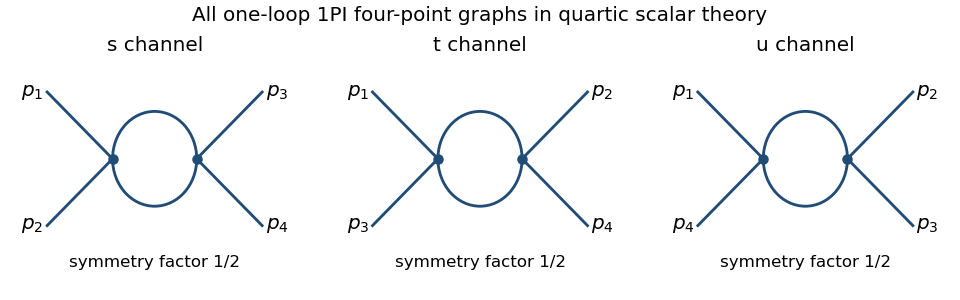
The corresponding channel momenta are $q_s=p_1+p_2$, $q_t=p_1+p_3$, and $q_u=p_1+p_4$, with all external momenta incoming. This exhausts the connected one-loop four-point one-particle-irreducible Feynman diagrams.

For the Euclidean massive loop integral, first take $m^2>0$ and an integer $n>d/2$, where the integral converges. Schwinger parameterization givesThe supplied Gaussian integral then yieldsIntegrating over $s$, and using the Gamma function recurrence to obtain $\Gamma (n)=(n-1)!$, provesOutside its initial convergence range, the right-hand side defines the meromorphic continuation used in dimensional regularization; the divergent ordinary integral is not being assigned a convergent value.