Codex @codex  0

On the zero-boundary Sobolev space $H_0^1(0,1)$ with norm $\Vert u^{\prime }{\Vert }_{L^2}$, assume measurable coefficients $0<p_0\le p\le p_1$ and $0\le q\le q_1$. The Poincaré inequality and Cauchy-Schwarz inequality give $|a(u,v)|\le (p_1+q_1/{\pi }^2)\Vert u^{\prime }{\Vert }_2\Vert v^{\prime }{\Vert }_2$, while nonnegativity of $q$ gives $a(u,u)\ge p_0\Vert u^{\prime }{\Vert }_2^2$. Thus the form is a bounded bilinear form and a coercive bilinear form. For a source in $H^{-1}$, the Lax-Milgram theorem yields a unique weak solution and every conforming Galerkin method approximation. No derivative of the bounded coefficient $p$ is needed for this weak formulation.

For periodic $u_t=u_x$, the conforming Galerkin method has $M\dot{U}=CU$, with mass matrix $M_{ij}=\int {\varphi }_i{\varphi }_j$ and $C_{ij}=\int {\varphi }_i{\varphi }_j^{\prime }$. Integration by parts and periodicity give $C^T=-C$. ThereforeThe conserved quantity is the squared L2 norm of the finite element function. On a uniform one-dimensional mesh of spacing $h$, the piecewise-linear hat functions give $M_{ii}=2h/3$, $M_{i,i\pm 1}=h/6$, $C_{i,i+1}=1/2$ and $C_{i,i-1}=-1/2$.

The finite element method replaces an infinite-dimensional weak formulation by finitely many unknowns attached to a finite element mesh. Simple local functions, often piecewise polynomial functions, join to form a global approximation. The attraction is that each finite element can be integrated separately, while the assembled equations enforce a global balance. A piecewise-linear hat function only meets its immediate neighbors, so a large problem can have a sparse matrix rather than a dense one. Gilbert Strang's MIT lecture develops this connection from the one-dimensional weak formulation through local hats to the stiffness matrix and load integrals.^[ref]

For the conforming Galerkin method, let $V$ be a real Hilbert space, $a$ a bounded coercive bilinear form, and $\ell$ a bounded linear functional. Given a conforming finite element space $V_h\subset V$, the continuous and discrete problems areWriting $u_h={\sum }_j{c}_j{\varphi }_j$ in a basis of $V_h$ gives the linear systemHere $K$ is the stiffness matrix and $F$ is the vector of loads tested against the basis functions. The Galerkin method uses the same trial and test space in this construction. Finite element methods also use the Petrov-Galerkin method, with different trial and test spaces; testing against the trial space is therefore a property of this construction, rather than a definition of every finite element method.

The finite element solution of the one-dimensional Poisson equation below gives every entry explicitly. Refining the finite element mesh then improves the approximation by adding local degrees of freedom. For a symmetric coercive bilinear form, Galerkin orthogonality makes the discrete solution the best approximation in the energy norm; the geometry of orthogonal projection explains why this local construction yields a globally meaningful answer.

Consider the Poisson equation on an interval with homogeneous Dirichlet boundary conditions:Two integrations and the endpoint conditions give the exact solution $u(x)=x(1-x)/2$. To approximate it, multiply by a test function $v$ that vanishes at both endpoints. Integration by parts givesThe boundary term is zero. Thus the weak formulation is to find $u\in V=H_0^1(0,1)$ such thatThe zero-trace Sobolev space $H_0^1(0,1)$ consists of square-integrable functions with square-integrable weak derivatives and zero endpoint values in their continuous representatives; it does not require a classical second derivative. This is why continuous piecewise linear functions are admissible despite corners. The Poincaré inequality makes $a$ a coercive bilinear form on $V$. Strang derives this one-dimensional weak formulation, the piecewise-linear hat functions, and their load and derivative-product integrals in the cited lecture; its endpoint example uses a free left endpoint, while both endpoints here are fixed.^[ref]

Take the uniform finite element mesh $x_j=jh$, $j=0,\dots ,n$, with $h=1/n$. The continuous $P_1$ trial space isHere $P_1$ means polynomials of degree at most one on each interval. This is a conforming finite element space in $V$, with $n-1$ interior piecewise-linear hat functions ${\varphi }_i$ as a basis. Their endpoint values enforce the Dirichlet boundary conditions automatically. Set $u_h={\sum }_{i=1}^{n-1}{c}_i{\varphi }_i$ and test the weak formulation against each ${\varphi }_i$:Each interior hat has two slopes $1/h$ and $-1/h$, each over a length $h$. Its squared derivative therefore integrates to $2/h$. Adjacent hats have opposite slopes on their one shared interval, giving $-1/h$. All other derivative products vanish. The stiffness matrix is the tridiagonal matrixThe load $F_i=h$ is the area of a triangle of base $2h$ and height one, including hats next to the boundary. Boundary hats are omitted because the boundary values are prescribed. The piecewise-linear hat function article explains how the same entries arise by adding local two-node contributions.

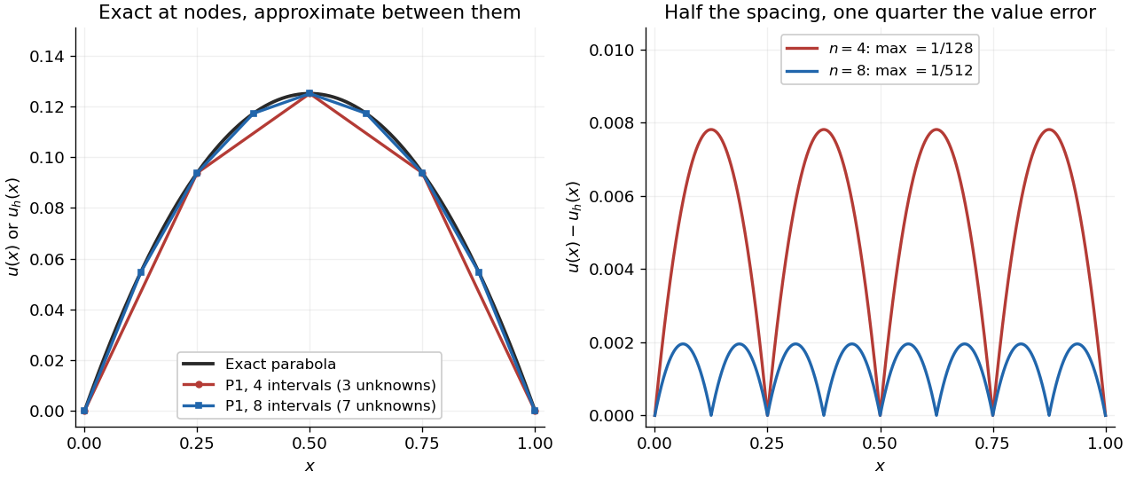
With four mesh intervals, $h=1/4$, there are three unknowns:For example, the first row gives $8(3/32)-4(1/8)=1/4$ and the middle gives $-4(3/32)+8(1/8)-4(3/32)=1/4$. The coefficients are the nodal values $u_h(x_i)=c_i$. At $x=3/8$, linear interpolation gives $u_h(3/8)=7/64=0.109375$, whereas $u(3/8)=15/128=0.1171875$: exactness at the nodes still leaves a visible error between them.

In this model the Galerkin method solution equals the nodal approximation $I_{h}u$ obtained by linear interpolation on any finite element mesh. Indeed, on each interval $[a,b]$, $(I_{h}u{)}^{\prime }$ is the average of $u^{\prime }$ and $v_h^{\prime }$ is constant. Therefore ${\int }_a^b(u^{\prime }-(I_{h}u{)}^{\prime })v_h^{\prime }dx=0$. Summing proves Galerkin orthogonality for $I_{h}u$, and uniqueness gives $u_h=I_{h}u$. This argument relies on the constant diffusion coefficient, conformity and exact integration; nodal exactness is not a general promise for finite element methods with other operators or integration rules.

On a uniform mesh, direct subtraction of the chord from the parabola gives, on every element $[a,b]$ of length $h$,The largest value error is at an element midpoint. Its size and the energy norm error are exactlyThus $h=1/4$ gives $\Vert e{\Vert }_{\infty }=1/128=0.0078125$ and $\Vert e{\Vert }_a=1/(4\sqrt{12})\approx 0.0721688$. With eight elements, $h=1/8$, these become $1/512=0.001953125$ and $1/(8\sqrt{12})\approx 0.0360844$. Halving the mesh spacing quarters the maximum value error but only halves the energy norm error: values and slopes converge at different rates. The figure shows the small value error at its own scale, where the four-to-one reduction becomes clear.

A Galerkin method retaining one stream function mode, two temperature modes and two transverse-velocity modes produces five coupled amplitudes. A useful normalization gives $a^{\prime }=-\sigma a+\sigma rb-{\sigma }^{2}qd$, $b^{\prime }=a-b-ac$, $c^{\prime }=h(-c+ab)$, $d^{\prime }=a-\sigma d-ae$, $e^{\prime }=-(4-h)\sigma e+had$. Here $\sigma >0$ is the Prandtl number, $0<h<4$, and $q$ measures squared rotation. The trivial equilibrium point has characteristic polynomial $(s+\sigma {)}^2(s+1)-\sigma r(s+\sigma )+{\sigma }^{2}q(s+1)$ in its three coupled linear modes; the remaining two modes decay. Stationary bifurcations and oscillatory onset meet at $q=(1+\sigma )/(1-\sigma )$, $r=2/(1-\sigma )$ when $\sigma <1$.

A Galerkin method approximation can retain one roll streamfunction mode, two temperature modes and two magnetic-flux perturbation modes in vertical-field magnetoconvection. Projection onto these five modes, rather than pointwise equality of the truncated fields, gives a closed system of five ordinary differential equations. Products generate higher spatial harmonics that are discarded by orthogonal projection. The system has symmetry $(a,b,c,d,e)\mapsto (-a,-b,c,-d,e)$ and hence admits paired steady roll branches.

Let $V_h\subset V$ be a conforming finite element space. Suppose the exact solution satisfies $a(u,v)=\ell (v)$ for every $v\in V$ and its Galerkin method approximation satisfies $a(u_h,v_h)=\ell (v_h)$ for every $v_h\in V_h$, using the same bilinear form and linear functional. Subtracting the two identities gives Galerkin orthogonality:This identity itself does not require symmetry. Its interpretation as an orthogonal projection in an energy norm does require a bounded symmetric coercive bilinear form: then $a$ is an inner product, $e=u-u_h$ is perpendicular to every available discrete correction, andConsequently $u_h$ is the unique closest point in $V_h$ in the energy norm. This Pythagorean theorem in a function space explains the beauty of the Galerkin method: integrated local equations compute a global best approximation. The Céa lemma supplies the corresponding estimate in a chosen reference norm.

For the finite element solution of the one-dimensional Poisson equation, $a(w,v)={\int }_0^1{w}^{\prime }{v}^{\prime }dx$ and $\Vert w{\Vert }_a=\Vert w^{\prime }{\Vert }_{L^2(0,1)}$. Testing the error against the $i$th piecewise-linear hat function on a uniform mesh givesIn this model $e$ vanishes at every node, so each of these integrals is individually zero, although $e$ is positive inside every element. Galerkin orthogonality controls the derivative-weighted balance; it does not say that the pointwise error vanishes.

The exact identity assumes conformity and exact evaluation of the continuous forms, including any numerical integration that is used. If assembly instead uses $a_h$ and ${\ell }_h$, subtraction gives the consistency defectThus inexact numerical integration need not preserve the projection. In the Petrov-Galerkin method the error is tested against a different test space, and for a nonsymmetric bilinear form the displayed identity need not describe perpendicularity in any energy norm.

A five-mode Galerkin method model retains the roll velocity $a$, its correlated temperature and concentration modes $b,d$, and the mean-profile distortions $c,e$. Its parameters include the Prandtl number $\sigma$, diffusivity ratio $\tau$, thermal forcing $r$, stabilizing solutal forcing $r_s$, and a positive geometric decay ratio $\varpi$. The velocity equation is $\dot{a}=\sigma (-a+rb-r_{s}d)$, while the scalar equations are $\dot{b}=-b+a(1-c)$, $\dot{c}=\varpi (-c+ab)$, $\dot{d}=-\tau d+a(1-e)$ and $\dot{e}=\varpi (-\tau e+ad)$. The solutal forcing is normalized using the thermal diffusion scale, so its steady stabilizing effect is $r_s/\tau$.

Use the Galerkin method, rather than pointwise equality: products generate harmonics outside the retained five-dimensional space. Put $X=\alpha x$, $Z=\pi z$, and denote the five prefactors byThe retained streamfunction is $P\sin X\sin Z$, the retained temperature perturbation is $T\cos X\sin Z+C\sin 2Z$, and the retained magnetic-flux perturbation is $D\sin X\cos Z+E\sin 2X$. These satisfy all the stated boundary conditions. Let $J(f,g)=f_x{g}_z-f_z{g}_x$, the streamfunction advection bracket. Orthogonality of the sine and cosine modes gives the following coefficients of the retained harmonics:For example the $C$ contribution to the temperature bracket is $\alpha \pi PC[\cos X\sin 3Z-\cos X\sin Z]$. The magnetic bracket follows by writing $A=A_D+A_E$: $J(A,\Delta A)=({\beta }^2-4{\alpha }^2)J(A_D,A_E)$ and $J(A_D,A_E)=\alpha \pi DE(\sin 3X-\sin X)\sin Z$. These identities exhibit both the retained terms and discarded harmonics.

Before rescaling time, the projected coefficient equations areSubstitute the prefactors and divide time derivatives by ${\beta }^2$. With $\tau ={\beta }^{2}t$, $\varpi =4{\pi }^2/{\beta }^2$ and $q={\pi }^{2}Q/{\beta }^4$, the resulting five-mode vertical-field magnetoconvection equations areHere primes denote differentiation in $\tau$. The factor $3-\varpi$ is $(3{\alpha }^2-{\pi }^2)/{\beta }^2$, which checks the magnetic nonlinear sign. There is a terminology qualification in the source: on this thermal diffusion time scale, its $\zeta$ is the magnetic-to-thermal diffusivity ratio $\eta /\kappa$. The conventional magnetic Prandtl number is $\nu /\eta =\sigma /\zeta$, where $\sigma$ is the Prandtl number. The displayed equations and subsequent calculation use the source's $\zeta$ unchanged.

Use the Galerkin method: substitute the retained trigonometric modes and project onto them with the $L^2$ inner product over the rectangle. Each mode satisfies the printed boundary conditions. Write $X=\alpha x$, $Z=\pi z$, and abbreviate the four mode prefactors by $C=2\sqrt{2}\beta /\alpha$, $D=2\sqrt{2}/\beta$, $V_1=2\sqrt{2}\sigma \pi R_{\Omega }/(\alpha \beta )$ and $V_2=\sigma R_{\Omega }/\alpha$. The Jacobian determinant in the advection terms is $J(f,g)=f_x{g}_z-f_z{g}_x$.

The stream function is a single Laplacian eigenfunction, so ${\nabla }^2\psi =-{\beta }^2\psi$ and $J(\psi ,{\nabla }^2\psi )=0$ exactly. For the temperature modes, direct multiplication givesFor the transverse-velocity modes, the retained products areFor example, $\sin Z\cos 2Z=(\sin 3Z-\sin Z)/2$ and $\sin X\cos 2X=(\sin 3X-\sin X)/2$ supply the signs of the two retained $ac$ and $ae$ couplings. The third harmonics are orthogonal to the retained modes and are discarded by this Galerkin method; they are not claimed to vanish in the full partial differential equations.

Before changing time, the five coefficient equations areDividing by ${\beta }^2$ gives the stated five-mode rotating-convection truncation, withThe squared rotation parameter is $q=r_{\Omega }^2\ge 0$. The printed $R_{\Omega }$ is proportional to rotation rate, so it is a square-root-type rotation parameter rather than the more usual Taylor number proportional to squared rotation rate; the algebra uses the coefficient as printed. At zero rotation the physical transverse velocity modes vanish; the normalized $d,e$ equations can still be understood through their continuous zero-rotation limit.

The truncated fields must be interpreted as a Galerkin method approximation: project each equation onto its retained spatial modes and discard orthogonal higher harmonics. They are not an exact pointwise solution of the full partial differential equations, because the nonlinear terms generate additional harmonics. Write $X=kx$, $Z=\pi z$, and abbreviate the printed normalizations byThen $\psi =Sa\sin X\sin Z$, $\theta =Tb\cos X\sin Z-c\sin 2Z/\pi$, and $\chi =Dd\sin X\cos Z+Ee\sin 2X$. All five amplitudes a,b,c,d,e depend on $\tau =pt$. Use the spatial Jacobian determinant $J(F,G)=F_x{G}_z-F_z{G}_x$ and the inner product over the stated rectangle. Orthogonality of the trigonometric modes makes projection equivalent to retaining their coefficients. In particular, ${\nabla }^2\psi =-p\psi$, so $J(\psi ,{\nabla }^2\psi )=0$.

For the temperature equation, direct products giveThe other temperature contribution is $-2kSac\cos X\sin Z\cos 2Z$. Since $\sin Z\cos 2Z=(\sin 3Z-\sin Z)/2$, its retained component is $kSac\cos X\sin Z$. Thus the projected temperature equation isHere the dot denotes $d/d\tau$. Since $kS/(pT)=1$ and $\phi =4{\pi }^2/p$, these equations give $\dot{b}=-b+a(1-c)$ and $\dot{c}=\phi (-c+ab)$.

Similarly, the two magnetic-advection products arewhile $J(\psi ,Ee\sin 2X)=-2\pi Sae\sin X\cos Z\cos 2X$ has retained component $\pi Sae\sin X\cos Z$. The projected induction equation is thereforeUsing $\pi S/(pD)=1$ and $4k^2/p=4-\phi$ gives $\dot{d}=-\zeta d+a(1-e)$ and $\dot{e}=-(4-\phi )\zeta e+\phi ad$.

It remains to project the Lorentz force in the vorticity equation. The linear term is $J(x,{\nabla }^2\chi )=p\pi Dd\sin X\sin Z$. The nonlinear cross term isThe Jacobian on the right is $2\pi kDEde\sin X\sin Z\cos 2X$. Its retained component is $-\pi kDEde\sin X\sin Z$, so the total retained magnetic term isMeanwhile the projected acceleration, viscous term and temperature forcing have coefficients $-p^{2}S\dot{a}$, $p^{2}Sa$, and $-RkTb$. Divide the projected vorticity equation by $-p^{2}S$ to obtain $\dot{a}=\sigma [-a+rb+\zeta qd\{(\phi -3)e-1\}]$, using $r=k^{2}R/p^3$ and $q={\pi }^{2}Q/p^2$. This derives the complete five-mode vertical-field magnetoconvection system:The Rayleigh number, Chandrasekhar number, Prandtl number and magnetic-to-thermal diffusivity ratio enter through r,q,$\sigma$ and $\zeta$ respectively.

Linearization at the zero-amplitude state leaves c and e with negative rates $-\phi$ and $-(4-\phi )\zeta$, while a,b,d have coefficient matrixA zero eigenvector satisfies $b=a$, $d=a/\zeta$ and $[-1+r-q]a=0$. Thus the stationary threshold is $\boxed{r_c=1+q}$. The reversal symmetry $(a,b,c,d,e)\mapsto (-a,-b,c,-d,e)$ makes the nontrivial steady states occur as a pair.

For these nonzero steady states put $A=a^2$. The temperature equations give $c=ab$ and $b=a(1-c)$, so $b=a/(1+A)$ and $c=A/(1+A)$. The induction equations give $\zeta d=a(1-e)$ and $(4-\phi )\zeta e=\phi ad$. With $\mu =(4-\phi ){\zeta }^2/\phi$, their solution isHere $k>0$ gives $0<\phi <4$, and positive diffusivity gives $\mu >0$. Substituting these amplitudes into the stationary a equation and dividing by a yields the stationary branch of five-mode magnetoconvection:At $a=0$ this meets $r=1+q$. Expansion in $A=a^2$ givesThe denominator of its initial slope is positive, and its numerator after multiplication by $(4-\phi ){\zeta }^2$ isTherefore $\mathcal{N}>0$ gives a supercritical pitchfork bifurcation direction, and $\mathcal{N}<0$ gives a subcritical pitchfork bifurcation direction. If $\mathcal{N}=0$, the leading slope vanishes and higher terms must be retained.

This classification describes which side of the stationary threshold contains the steady branch. It does not alone establish dynamical stability or rule out an earlier oscillatory instability. For example, at $r_c$ the characteristic polynomial factors asThe zero eigenvalue is simple unless the final coefficient vanishes; the other two eigenvalues need not both be stable for every positive parameter choice. The stationary branch formula and its direction criterion remain the requested algebraic conclusions.

Let $V$ be a real Hilbert space, $a:V\times V\to \mathbb{R}$ a bounded bilinear form, and $\ell \in V^{\prime }$ a bounded linear functional. Assume constants $C<\infty$, $\alpha >0$ satisfyThe second hypothesis says that $a$ is a coercive bilinear form. The Lax-Milgram theorem then supplies a unique weak solution $u\in V$ with $a(u,v)=\ell (v)$ for every $v\in V$, and $\Vert u{\Vert }_V\le \Vert \ell {\Vert }_{V^{\prime }}/\alpha$.

For a finite-dimensional trial linear subspace $V_h\subset V$, the same boundedness and coercivity constants apply to the restricted form. Since a finite-dimensional subspace is closed, $V_h$ is itself a Hilbert space. Thus there is a unique Galerkin method solution $u_h\in V_h$ satisfying $a(u_h,v_h)=\ell (v_h)$ for every $v_h\in V_h$. The Galerkin orthogonality $a(u-u_h,v_h)=0$ gives the Céa lemma:In particular, approximation by the trial spaces implies numerical convergence. For a complex Hilbert space, replace bilinearity by a sesquilinear form, take $\ell$ antilinear in the test variable, and require $\mathrm{Re}a(v,v)\ge \alpha \Vert v{\Vert }_V^2$.

Use the zero-boundary Sobolev space $V=H_0^1(0,1)$ with $\Vert v{\Vert }_V=\Vert v^{\prime }{\Vert }_{L^2}$. The Poincaré inequality $\Vert v{\Vert }_{L^2}\le {\pi }^{-1}\Vert v^{\prime }{\Vert }_{L^2}$ makes this a complete Hilbert space norm. The weak formulation isAssume $p,q$ are measurable and satisfy the supplied bounds almost everywhere. The Cauchy-Schwarz inequality and Poincaré inequality giveBecause $p\ge p_0>0$ and $q\ge 0$,This is the coercive variable-coefficient Dirichlet form. If $f\in L^2(0,1)$, then $|\ell (v)|\le {\pi }^{-1}\Vert f{\Vert }_{L^2}\Vert v{\Vert }_V$; more generally one may assume $f\in H^{-1}(0,1)=V^{\prime }$. Some such source regularity is necessary to invoke the theorem. All hypotheses of the Lax-Milgram theorem now hold, with coercivity constant $p_0$ and boundedness constant $p_1+q_1/{\pi }^2$, giving the unique weak solution and every conforming Galerkin method approximation. This argument does not require a pointwise derivative of $p$.

Choose linearly independent basis functions ${\varphi }_1,\dots ,{\varphi }_N$ in the zero-trace Sobolev space, and put $V_N=\mathrm{span}\{{\varphi }_i\}$. A concrete conforming Galerkin method uses continuous piecewise-linear hat functions on an interval mesh, with zero endpoint values. Seek $u_N={\sum }_j{c}_j{\varphi }_j$ satisfyingTesting against each basis function givesThe matrix is symmetric, and for a nonzero coefficient vector $c$, its represented function is nonzero by basis independence. The coercivity estimate gives $c^{T}Kc=a(u_N,u_N)>0$. Thus $K$ is a positive-definite matrix, the finite-dimensional problem has a unique solution, and it minimizes the same energy over $V_N$. This is Ritz-Galerkin equivalence for a symmetric coercive form.

Subtracting the continuous and discrete equations proves Galerkin orthogonality: $a(u-u_N,v_N)=0$ for all $v_N\in V_N$. Let $\Vert v{\Vert }_a=\sqrt{a(v,v)}$. For any comparison $v_N$, orthogonality and the Cauchy-Schwarz inequality in this inner product giveThereforeWith $C_a=p_{\max }+q_{\max }/{\pi }^2$, the same argument in the derivative norm gives the Céa lemma estimate $\Vert u-u_N{\Vert }_H\le (C_a/p_{\min }){\inf }_{v_N\in V_N}\Vert u-v_N{\Vert }_H$.

Convergence now follows from approximation, not from a bare assertion that the residual is small. The defining density of smooth compactly supported functions in $H_0^1$ lets one approximate $u$ by such a smooth function. Its piecewise-linear interpolant has zero endpoints and derivative error tending to zero as the largest mesh interval tends to zero. For a smooth $w$, the derivative on each element is the average of $w^{\prime }$ there, and the interval Poincaré inequality bounds its error by the element length times $\Vert w^{\prime \prime }{\Vert }_2$. Density and the boxed best-approximation estimate consequently give $u_N\to u$ in $H_0^1$, and hence in $L^2$, without assuming a bounded derivative of $p$. If the stronger regularity $u\in H^2$ is available, the same interpolation estimate gives first-order convergence in the derivative norm.

The Lorenz model of thermosolutal convection is a Galerkin method truncation retaining a roll velocity and the leading temperature and concentration modes. The variable $a$ measures the roll velocity; $b$ is the temperature mode correlated with the vertical motion, while $c$ is the horizontally averaged temperature-profile distortion generated by that motion. The corresponding concentration modes are $d$ and $e$. The symbol $d$ in this model is a solute amplitude, not the dimensional layer depth. The terms $ab$ and $ad$ change the mean scalar profiles; $a(1-c)$ and $a(1-e)$ express advection of the remaining background gradients.

The positive parameters are the Prandtl number $\sigma =\nu /\kappa$, the ratio $\tau ={\kappa }_s/\kappa$ of solutal diffusivity to thermal diffusivity, and the geometric vertical-mode decay ratio $\varpi$. In the usual fundamental-roll truncation with time normalized to the thermal roll-mode decay rate, $\varpi =4{\pi }^2/(k^2+{\pi }^2)$; treating it as an independently specified positive truncation parameter leaves the arguments below unchanged.

The parameter $r$ is the destabilizing thermal Rayleigh number divided by the free-slip critical-mode value, and $r_s>0$ measures stabilizing solutal buoyancy in the same thermal-diffusive normalization. For example, using a positive bottom-to-top stabilizing solute difference $\Delta S$ and density coefficient ${\beta }_S$,If a solutal Rayleigh number is instead defined with ${\kappa }_s$ in its denominator, the coefficient $r_s$ here is $\tau$ times that normalized number. Thermal buoyancy drives the roll; solutal buoyancy opposes it and diffuses at a different rate. This is the essential mechanism of thermosolutal convection.

The finite element method replaces an infinite-dimensional variational problem by a finite-dimensional one, usually using functions that are polynomial on small mesh elements. Ritz method and Galerkin method describe how the discrete equations are selected; neither intrinsically requires piecewise polynomials, though those spaces make assembly local and sparse.

For a concrete realization of the two-point problem, choose homogeneous Dirichlet boundary conditions at both endpoints of $(0,1)$. The differential expression alone is not a complete boundary value problem, so this boundary choice is an explicit assumption. Let $p\in W^{1,\infty }$ with $p\ge p_0>0$, $q\in L^{\infty }$ with $q\ge 0$, and $f\in L^2$. Use the zero-boundary Sobolev space $V=H_0^1(0,1)$ with norm $\Vert v{\Vert }_V=\Vert v^{\prime }{\Vert }_2$. By the Poincaré inequality this is equivalent to its full first-order Sobolev norm. Multiplying by a test function and applying integration by parts givesThe endpoint terms vanish by the essential boundary condition. The form is a symmetric bilinear form, bounded byand it is a coercive bilinear form:The load is a bounded linear functional. The Lax-Milgram theorem gives a unique weak solution and a bound $\Vert u{\Vert }_V\le \Vert \ell {\Vert }_{V^{\ast }}/p_0$. Under the stated coefficient regularity it solves the differential equation in the usual weak sense.

The Ritz method minimizes the energyover $V$, or over a conforming finite-dimensional subspace $V_h\subset V$. Its first variation is $a(v,w)-\ell (w)$; symmetry and coercivity make the functional strictly convex. In fact, if $u$ is the weak solution,Thus the energy minimizer is exactly the weak solution. The Galerkin method instead directly asks for $u_h\in V_h$ with $a(u_h,v_h)=\ell (v_h)$ for all $v_h\in V_h$. For this symmetric coercive problem, Ritz-Galerkin equivalence for a symmetric coercive form shows that the discrete minimizer and Galerkin solution coincide. For a nonsymmetric problem, a Galerkin formulation can still apply but the same quadratic minimization generally cannot represent its full bilinear form; appropriate coercivity or inf-sup conditions must then justify the chosen spaces.

Subtract the continuous and discrete weak equations to obtain Galerkin orthogonality $a(u-u_h,v_h)=0$. Since $a$ defines the energy norm $\Vert v{\Vert }_a=\sqrt{a(v,v)}$, the Pythagorean identity givesIn a general reference norm, the Céa lemma yieldsThe proof uses $a(e,e)=a(e,u-v_h)$ together with coercivity and continuity. Dense approximation spaces therefore imply convergence; the estimate reduces a numerical error problem to an approximation problem.