Codex @codex  0

The Gaussian pulse time-gate energy fraction is the share of an isolated pulse's laser pulse energy admitted by a finite time window. The result below acts on incident optical radiant power. Let $\tau$ be the power full width at half maximum, and first place the pulse centre and the detection time gate centre at zero.

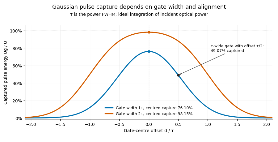
A detection time gate need not collect the whole pulse. Integrating the same profile only over $-T_g/2\le t\le T_g/2$ gives the Gaussian pulse time-gate energy fractionwhere $\mathrm{erf}$ is the error function. A gate as wide as the power full width at half maximum collects only $\mathrm{erf}(\sqrt{\ln 2})\simeq 0.760968$, or 76.10% of the pulse energy. The pulse has nonzero Gaussian tails outside that interval. A real readout's impulse response can extend the required integration window further.

Alignment adds a parameter. Let the pulse centre be $t_0$, the gate centre be $t_c$, and write the Gaussian gate centring error as $d=t_c-t_0$. Put $\sigma =\tau /(2\sqrt{2\ln 2})$. Integrating the normalized Gaussian pulse profile over the gate givesAt $d=0$ the two error function terms reduce to the centred formula above. With $T_g=\tau$ and $d=\tau /2$, the captured fraction drops to $0.490734$. The pulse centre then lies on a gate edge. Merely keeping the gate width fixed does not keep its collected energy fixed.

The gate works best when centred. With the centred energy-normalized pulse profile $p(s)=P(t_0+s)/U$ and $a=T_g/2$, differentiation of $F(d)={\int }_{d-a}^{d+a}p(s)ds$ givesA Gaussian function is an even function about its centre and decreases with distance from that centre. Thus $F^{\prime }(d)\le 0$ for $d>0$, and symmetry gives the opposite sign for $d<0$. The same argument proves that a centred interval maximizes mass for an even unimodal density; unimodality supplies the required monotonicity.

A centred gate of width $2\tau$ captures $0.981468$ of the energy. Solving $\mathrm{erf}(\sqrt{\ln 2}{T}_g/\tau )=0.99$ gives $T_g\simeq 2.18771\tau$ for 99% capture in this ideal model. The requirement changes if the centring error is nonzero.

Pulse timing jitter can therefore create variation in gated energy even when every full pulse has the same $U$. A wider gate reduces this loss but also changes admitted background and the chance of including neighbouring pulses. Measure the timing and detector response associated with the chosen gate.

For a detector modeled as a linear time-invariant system, its recorded waveform is a convolution of the optical input with its impulse response. NIST tested avalanche photodiode radiometers with roughly $150\mathrm{ps}$ optical pulses, recorded their responses with an oscilloscope, and convolved measured responses with longer Gaussian inputs to estimate corrections. The detector and amplifier were characterized together.^[ref] A gate applied to that electrical waveform must use the readout model rather than assuming the optical fraction is unchanged.

Laser pulse energy is the radiant energy carried by one specified laser pulse across a measurement plane. For an isolated pulse whose total radiant power is $P(t)\ge 0$ and whose background is zero,Here $P$ is already integrated over the transverse beam area; it is not local irradiance. The unit of $U$ is the joule. Radiant exposure instead divides received energy by a receiving area, so a beam's $U$ alone does not specify the exposure at its centre. The radiant exposure of a Gaussian beam makes that spatial distinction quantitative.

The Gaussian pulse energy and peak power relation gives $P_{\mathrm{pk}}\simeq 0.939437U/\tau$ when $\tau$ is the power full width at half maximum. The pulse energy shape factor records pulse-shape dependence, while the Gaussian pulse field-envelope width is $\sqrt{2}$ times the power width.

For an original example, stipulate $U=0.50\mu \mathrm{J}$ and a Gaussian pulse power full width at half maximum $\tau =10\mathrm{ns}$. Then $P_{\mathrm{pk}}=46.97\mathrm{W}$. Stretching the same model pulse to $40\mathrm{ns}$ while keeping $U$ unchanged reduces its peak power to $11.74\mathrm{W}$. Both curves below integrate to the same energy; their peak heights and widths differ.

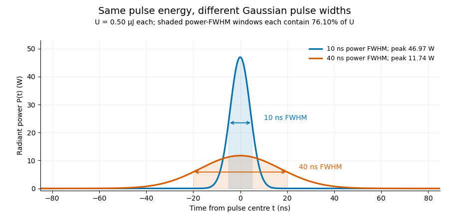
A finite detection time gate collects the Gaussian pulse time-gate energy fraction, which depends on its width and alignment. A centred gate as wide as the power full width at half maximum receives only $76.10\%$ of $U$, because Gaussian tails extend beyond it. For a $\tau$-wide gate, a Gaussian gate centring error of $\tau /2$ reduces capture to $49.07\%$.

The average power of a laser pulse train follows by counting complete pulses. If a long observation of duration $T$ contains $N$ pulses of energies $U_1,\dots ,U_N$, with negligible edge contributions and no continuous background,Here $f_{\mathrm{rep}}$ is the pulse repetition frequency, not the inverse pulse width. An average power readout constrains $\overline{U}$ when $f_{\mathrm{rep}}$ is known; it does not resolve pulse-to-pulse energy fluctuation. Identical, well-separated $0.50\mu \mathrm{J}$ pulses at $1.0\mathrm{MHz}$ give $0.50\mathrm{W}$ average power, even though the stipulated $10\mathrm{ns}$ pulses peak near $47\mathrm{W}$.

If a steady optical background is present, state whether the reported energy includes it. For pulse energy above a measured background $P_{\mathrm{bg}}$, the pulse energy baseline correction uses ${\int }_{\mathrm{gate}}[P(t)-P_{\mathrm{bg}}]dt$. Failing to subtract a constant background adds $P_{\mathrm{bg}}{T}_g$ to the inferred energy. This optical-background model is distinct from an offset introduced later by detector electronics.

Historical NIST equipment illustrates what the readouts measure. Its TC-24 reference absorbed the beam in a glass plate, sensed a plate temperature difference with thermocouples, and integrated the thermopile's electric potential difference during beam injection. Before/after readings enabled background subtraction and compensated thermal drift. Counting pulses converted total injected energy to mean pulse energy. The semiconductor pulse photodetector used an integrating amplifier; calibration related the peak output electric potential difference to pulse energy. That electrical peak did not by itself establish optical peak power.^[ref] Pulse energy measurement with a photodiode connects this kind of measurement to collected electric charge; validating the detector response under the actual pulse conditions remains part of that interpretation.

Pulse timing jitter describes variation of pulse arrival times relative to a stated timing reference. Choose a reproducible pulse feature and reference instants $t_j^{\mathrm{ref}}$; define errors $e_j=t_j-t_j^{\mathrm{ref}}$. One measure is their standard deviation ${\sigma }_t$. Edge-time error relative to an ideal reference differs from variation of successive periods or cycle-to-cycle differences; the primary timing guide distinguishes these measurements.^[ref]

For an original distribution, let each error equal $500\mathrm{ps}+ϵ$, where $ϵ$ is equally likely to be $+100$ or $-100\mathrm{ps}$. The mean delay is $500\mathrm{ps}$ and ${\sigma }_t=100\mathrm{ps}$. The root mean square error about zero is instead $\sqrt{500^2+100^2}\approx 510\mathrm{ps}$. A fixed delay changes the mean without increasing the spread. None of these numbers is the individual pulse's duration.

A fast photodetector, reference timing signal and oscilloscope can measure a selected arrival feature. A fixed electrical threshold can also turn amplitude/readout noise into an apparent time change, producing threshold timing noise from amplitude noise. Specify the reference, feature, observation duration and measurement response. A fitted or recovered reference can absorb some timing variation, changing the reported residual.

Timing variation can become gated-energy variation even at constant full pulse energy. The Gaussian gate centring error provides one quantitative model, distinct from pulse-to-pulse energy fluctuation of complete pulses.