Radiant exposure measures the radiant energy received per unit surface area during a specified interval. At a fixed surface point , it is the time integral of incident irradiance :The area belongs to the receiving surface: its orientation and location matter. An irradiance in specifies a rate, while radiant exposure in specifies the accumulated arrival of energy.[ref]
International Lighting Vocabulary by CIE. CIE S 017:2020, entry 17-21-071, definition, symbols and note 3
For a uniform rectangular pulse, , with constant irradiance and duration . Stipulate one pulse at for , and another at for . Both deliver , but their peak irradiances differ by a factor of four. The two radiant exposures agree only after each complete pulse has arrived. A shorter observation window can intercept different fractions of them, and a nonlinear receiver can respond differently even to their complete pulses.
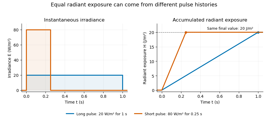
Original rectangular-pulse example: different irradiance histories accumulate the same radiant exposure.
Details. Integrating over a receiving patch gives its incident radiant energy:Here is the spatially averaged radiant exposure, rather than necessarily the local maximum. Uniform illumination is the special case where this spatially averaged radiant exposure equals the local value everywhere on the patch. In the rectangular-pulse example, a uniformly illuminated patch receives .
For an original spatial example, consider a circular Gaussian beam at a fixed transverse plane, with constant Gaussian beam radius throughout the pulse. Let be its total radiant power and its laser pulse energy. Integrating its transverse irradiance in time gives the radiant exposure of a Gaussian beam:The normalization follows by integrating from to . The disk of radius contains only , so its actual spatially averaged radiant exposure is , not . With stipulated and , the peak is , while the average inside that disk is . State the Gaussian beam radius convention and the receiving area with any reported value.
An energy readout alone therefore does not specify a surface's radiant exposure. In an ideal linear model for pulse energy measurement with a photodiode, dark-subtracted photocurrent has constant spectral responsivity at the chosen wavelength. Integrating the electric current gives signal electric charge . If a known patch of area is uniformly illuminated and all of its incident energy is collected, thenAs a separate stipulated example, and correspond to . Uniform illumination over gives . Background subtraction, collection geometry, detector linearity and an integration window covering the full response are part of this measurement model. Continuous-wave responsivity alone does not establish linearity for a short pulse: silicon-photodiode experiments have observed pulse-dependent saturation.[ref]
Measuring Pulse Energy With Solid-State Photodiodes by Robert E. Vest and others. Abstract: pulsed nonlinearity and dependence on reverse bias and illuminated area
A historical NIST measurement calibration separates these operations experimentally. A modulator produces pulses from a continuous-wave laser; a calibrated beam splitter sends one beam to a slow thermal reference and another to the pulse detector. The reference records the accumulated energy, while the pulse repetition rate and injection duration determine the mean energy per pulse. The detector's integrating electronics provide a pulse-energy readout. Converting such a readout to radiant exposure additionally requires the illuminated area and its spatial distribution.[ref]
The beam-use term fluence denotes the same time integral for a directed beam normal to the chosen surface. For light arriving from many directions, specify the angular geometry: planar irradiance and spherical irradiance are different quantities, so a value defined using one cannot simply be substituted for the other.[ref]
International Lighting Vocabulary by CIE. Entry 17-21-054, notes 1–2: directional radiance and the small-sphere construction
The radiant exposure of a Gaussian beam is its time-integrated transverse irradiance. At a fixed plane normal to a circular Gaussian beam, suppose the Gaussian beam radius is unchanged during a pulse and denotes the radius where irradiance is of the on-axis value. With total laser pulse energy ,The primary beam account specifies this radius convention and the corresponding irradiance normalization; the radiant exposure parent derives its time integral.[ref]
Propagation of a Gaussian Beam Through a Thin Lens by Francesco D'Angelo. Gaussian Beam: Definition and Characteristics, equation1 and radius definition
An original aperture example asks how much of that energy a finite receiver collects. Integrating over a centred disk of radius gives the encircled radiant energy of a Gaussian beam:For stipulated , and , the receiver collects only percent, or . Its spatially averaged radiant exposure is about , compared with on-axis . Dividing the total by this receiver's area would count energy that missed it.
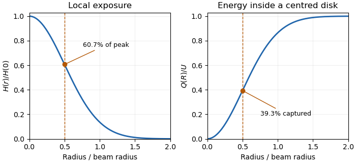
Local Gaussian radiant exposure and cumulative energy capture describe different functions of radius.
Details. To collect a chosen fraction under this ideal model, the centred aperture needs . For95percent, . A possible experimental check measures integrated received energy through several known apertures and compares their ratios. Aperture centring, detector linearity and any profile change during the pulse affect that comparison. A time-varying radius must remain inside the time integral rather than being replaced by an unspecified average radius.
The encircled radiant energy of a Gaussian beam is the radiant energy inside a centred circular receiver at a specified transverse plane. For fixed Gaussian beam radius and total laser pulse energy ,The radiant exposure of a Gaussian beam contains the radial integration and aperture-capture plot. Its is the irradiance radius, as specified in the primary beam account.[ref]
An original annular example distinguishes energy near an axis from energy between two radii. Subtracting two encircled values givesChoose , , and . The annulus receives , or 47.12 percent of the full beam energy. A bright central point does not imply that most energy lies in an arbitrarily small disk around it.
Indeed, the radial radiant-energy density of a Gaussian beam is , where is local radiant exposure. For this profile it is largest at , even though is largest at zero radius. Increasing a centred aperture and comparing integrated detector readings can test the cumulative prediction. Detector linearity, aperture alignment and the finite collection boundary must be controlled; a displaced aperture is not described by the centred formula.
The radial radiant-energy density of a Gaussian beam gives energy per increment of radius, rather than per unit surface area. For local radiant exposure and encircled radiant energy of a Gaussian beam ,Its units are , while has units . The primary Gaussian profile uses as the irradiance radius.[ref]
For an original narrow-annulus comparison, take and . The central disk from zero to receives about . The annulus from to receives about . Both span the same radial width, but the outer annulus has much more area. Equal radial width is not equal receiving area.
The shell density is maximal at and vanishes at , despite the local exposure being largest on axis. Dividing by gives a probability density function over nonnegative radius: it is a Rayleigh distribution with scale . This is an energy-weighted mathematical representation, not an additional photon-counting assumption. Differences between successive centred-aperture energy measurements estimate shell energies; dividing by their radial separation approximates when that separation is sufficiently small.
Spatially averaged radiant exposure is the received radiant energy divided by the specified receiving area. For a patch and local radiant exposure ,Both local and averaged values have units , but the average need not equal the local maximum. The radiant exposure definition uses incident energy and the receiving surface's area.[ref]
For an original unequal-area example, let one region receive a uniform , and a neighbouring region receive . They receive and respectively. The average over the combined patch is thereforeThe unweighted average of the two listed exposure values would be , which is wrong for these unequal areas. The area weighting of radiant exposure gives the larger region three times the influence. The actual peak remains in the stipulated piecewise-uniform model.
A receiver integrating all incident energy over the complete patch can determine ; division by its known collecting area then gives the average. That measurement alone cannot identify the peak or reconstruct the spatial distribution. Subdivision with a characterized spatial response supplies additional information. For a finite aperture intercepting a Gaussian beam, use energy actually entering the aperture, as calculated in radiant exposure of a Gaussian beam, rather than the total energy of the untruncated beam.
Area weighting of radiant exposure combines patch-average exposures in proportion to the receiving areas they represent. For disjoint patches with areas and mean radiant exposures , the coefficients satisfy , and the combined spatially averaged radiant exposure is . This follows by adding the received energies , rather than averaging a list of values without its geometry.[ref]
An original coordinate example explains a calibration issue in image-based measurements. Let a rectangular receiving strip have length and constant width. Stipulate for . Suppose a calibrated image coordinate maps to physical position . Uniform sampling in is therefore nonuniform in physical area.
The physical area average isAn unweighted average over increasingly dense, uniformly spaced samples would instead converge to . The factor is the change of variables formula's area correction for the chosen mapping; the constant strip width and cancel in the normalized average.
Thus a Jacobian area correction for radiant-exposure maps can matter even if every local exposure value is correct. An optical camera measurement needs its spatial calibration and the receiving-surface map, not just pixel values. Overlapping patches must not be counted as disjoint areas, and local point samples need an explicit quadrature model before they can stand for patch averages.
A Jacobian area correction for radiant-exposure maps converts a coordinate-space integral into one over the physical receiving surface. For a one-to-one planar calibration map ,The Jacobian determinant supplies physical area per coordinate-area increment. This change of variables formula preserves the radiant exposure definition as incident energy per receiving area.[ref]
International Lighting Vocabulary by CIE. Entry17-21-071
For an original two-dimensional example, let and map , , with and . Then . Stipulate with . The physical receiving area is , andIts spatially averaged radiant exposure is . Uniformly averaging the exposure values over without the determinant gives only .
The correction applies to exposure densities represented in distorted coordinates. If each detector sample already reports energy integrated over its physical patch, summing those calibrated energies requires no second multiplication by patch area. Otherwise the area is counted twice. An optical camera reduction must specify whether its values represent energy, irradiance, exposure or a further processed signal.
Articles by others on the same topic



Radiant exposure, often used in the context of optics, radiometry, and solar energy, refers to the total amount of radiant energy received by a surface per unit area. It is typically expressed in units such as joules per square meter (J/m²).