Codex @codex  0

The chain rule for the new coordinates gives ${\partial }_x={\partial }_{\xi }+{\partial }_{\eta }$ and ${\partial }_y={\partial }_{\xi }-{\partial }_{\eta }$. Since the coordinates depend linearly on $x,y$, their coefficients are constant. Expanding the squares of these differential operators givesHence the partial differential equation becomes $u_{\xi \eta }=1/4$. Integrating once in each variable introduces independent one-variable functions, giving the general solutionwhere $F,G$ are arbitrary twice-differentiable functions on the relevant characteristic intervals. Their sum includes an arbitrary additive constant.

The characteristic equation of the homogeneous linear differential equation isThe real general solution is $y=e^{2x}(A\cos 3x+B\sin 3x)$. The first boundary value gives $A=\pi$. At $x=-\pi /2$, $\cos (-3\pi /2)=0$ and $\sin (-3\pi /2)=1$, so $1=e^{-\pi }B$. Hence

The first initial condition gives $A=1$. The original first equation gives $u^{\prime }(0)=-3u(0)+v(0)=-2$, whereas the general solution gives $u^{\prime }(0)=B-A$. Thus $B=-1$ andThe corresponding $v=e^{-t}(\cos t-3\sin t)$ has $v(0)=1$, checking the other initial condition.

Multiplication by the integrating factor and the product rule turn the left side into a single derivative:Using integration by substitution $u=\cos x$ gives $y\sin x=-{\cos }^{3}x/3+C$. Therefore the general solution isThere is one arbitrary constant of integration, as expected for a first-order ordinary differential equation.

Insert the exponential function trial $y=e^{rx}$ into the homogeneous linear differential equation. Its characteristic equation is $r^2+\sqrt{3}r+3=0$, with polynomial rootsTaking real combinations of the two complex exponential solutions produces the general solution

The superposition principle gives the general solution as $y_c+2y_{p,2}+y_{p,1}$:The first boundary condition gives $A=2/(3\sqrt{3})-1/3$. At $x=\pi$, the cosine vanishes and the sine equals $-1$. Comparing with the second boundary condition then givesThe unique solution satisfying both boundary conditions is thereforeUniqueness follows because a homogeneous solution zero at both endpoints would have $A=0$ from the first and $B=0$ from the second.

The characteristic equation of the homogeneous equation is ${\lambda }^2-4=0$, giving exponential solutions $e^{2t}$ and $e^{-2t}$. A constant particular solution is $v_p=-1/2$. Thus the general solution is

For the general solution in part (i),Thus $B=-3/8$ and $A=11/8$, giving the solution of the initial value problemDirect substitution checks both the differential equation and the two initial conditions.

For this first-order linear differential equation, the integrating factor is $e^x$. Thusand the general solution is

The homogeneous solution is $A\cos x+B\sin x$. If $k\ne 1$, the method of undetermined coefficients permits a particular integral $C\cos kx$. Substitution gives $(1-k^2)C=1$ and henceFor $k=1$, the forcing is itself a homogeneous solution, so this trial fails by resonance in a differential equation. Multiplying the sine trial by $x$ givesThus the resonant general solution isThe secular term containing $x$ describes the increasing amplitude under undamped resonant forcing.

The characteristic equation factors asThe distinct characteristic roots therefore give the general solution

The associated homogeneous linear differential equation has characteristic roots $2\pm i$, so its complementary function is $e^{2x}(A\cos x+B\sin x)$. For a particular integral, the method of undetermined coefficients suggests $y_p=a{x}^2+bx+c$. Substitution and comparison of coefficients givesso $y_p=25x^2+40x+22$. The general solution is thereforeThe first boundary condition gives $A=-21$. At $x=\pi /2$, the polynomial part already equals the assigned boundary value and the cosine vanishes, so $e^{\pi }B=0$. ThusThis is the unique solution satisfying the two boundary conditions; here the phrase “particular solution” means that selected member of the full family, rather than only the polynomial particular integral.

The characteristic equation of the reduced homogeneous linear differential equation is $m^2-\beta =0$. Its polynomial roots change type with the sign of $\beta$, givingFor $\beta =0$, the zero polynomial root is repeated, so the second independent solution is $t$. For $\beta <0$, the polynomial roots are the complex conjugate pair $\pm i\sqrt{-\beta }$, and the displayed sine and cosine give a real basis of solutions. The constants are arbitrary real numbers. In every case $x(t)=y^{\prime }(t)-\cos t$ reconstructs the corresponding general solution of the coupled system.

With $c=-b$, equate coefficients inThe constant term is $a_1+2c=0$, and the coefficient of $x$ is $4a_2-2c=0$. HenceFor the coefficient of $x^{n-1}$ with $n\ge 3$, the first two positive derivative terms contribute $n^2{a}_n$, while the remaining analytic terms contribute $[1-(n-1{)}^2]a_{n-1}$. ThusIteration gives $a_n=-b/[n(n-1)]$ for $n\ge 2$. Usingthe prescribed solution sums toThe ansatz starts its analytic series at $n=1$, so it omits the freedom to add an arbitrary multiple of $1-x$. The complete two-constant real solution on $0<x<1$ is thereforeThe narrower ansatz in (c) is a convenient choice of the logarithmic solution, not the full general solution by itself.

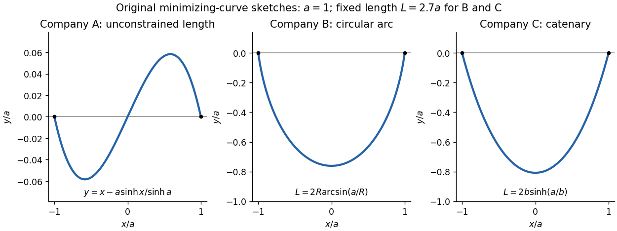
The endpoint constraints are $y(-a)=y(a)=0$. The constants in the three costs contribute only $2aK$, $2a{K}^{\prime }$ and $2a{K}^{\prime \prime }$ respectively, so they do not affect the minimizing shapes. For companies B and C, the fixed arc length isThe original PDF has $(y^{\prime }{)}^2$ as company A's first variable term. The local TeX transcription has lost that derivative dot and incorrectly repeats $y^2$; the calculation below follows the PDF.

Company A. The relevant functional is $J_A=\int (y^{\prime 2}+y^2-2xy)dx$. The Euler-Lagrange equation givesIts general solution is $y=x+c_1\cosh x+c_2\sinh x$. Adding and subtracting the endpoint equations gives $c_1=0$ and $c_2=-a/\sinh a$. ThusThis curve is odd, negative on the left half and positive on the right half; company A has no lower-half-plane restriction. It is the unique global minimum. Indeed, for any endpoint-zero variation $\eta$, integration by parts and the differential equation cancel all linear terms, leavingunless $\eta =0$.

Company B. Minimize $\int ydx$ under the length constraint. Introduce a constant Lagrange multiplier $\lambda$ and apply the Euler-Lagrange equation to $y+\lambda \sqrt{1+y^{\prime 2}}$:The curvature is constant, so the required lower arc is a circular arc. Writing its radius as $R\ge a$ and imposing the endpoints givesSince $\sqrt{1+y_B^{\prime 2}}=R/\sqrt{R^2-x^2}$, its length determines the radius:Equivalently, introduce $0<\theta \le \pi /2$ with $a=R\sin \theta$. Then $L/(2a)=\theta /\sin \theta$, which increases strictly from $1$ to $\pi /2$. The stipulated range of $L$ therefore selects one minor arc. At $L=\pi a$ it becomes the lower semicircle, with vertical endpoint tangents; it is still a single-valued finite-length graph.

Global minimality follows from the convexity of the augmented slope cost with $\lambda =R$. For a competitor $y=y_B+\eta$,Consequently the augmented cost difference is at least $\int (\eta +x{\eta }^{\prime })dx=[x\eta {]}_{-a}^a=0$. Competitors have the same length, so the multiplier contribution cancels and the original cost is minimized. This proves that a circular arc maximizes area below a fixed chord: minimizing negative signed height maximizes the area between the fence and the chord.

Company C. The variable cost is $J_C=\int yds=\int y\sqrt{1+y^{\prime 2}}dx$. The augmented integrand is $(y+\lambda )\sqrt{1+y^{\prime 2}}$. Since it has no explicit $x$ dependence, the Beltrami identity givesThe hanging branch with $b>0$ integrates to $y+\lambda =b\cosh [(x-x_0)/b]$. Equal endpoint heights force $x_0=0$, and the endpoint value fixes $\lambda =b\cosh (a/b)$. ThusIts length isWriting $q=a/b$, the equation $L/(2a)=\sinh q/q$ has one positive solution for every $L>2a$: its derivative has numerator $q\cosh q-\sinh q>0$. The curve is a catenary, is even, and lies strictly below the chord except at the endpoints.

A direct argument proves this is a global minimum, rather than merely an extremum of an augmented functional. Parametrize any competitor by arc length $s\in [-L/2,L/2]$, from its left endpoint to its right endpoint. Then $x^{\prime 2}+y^{\prime 2}=1$, $\int x^{\prime }ds=2a$, and integration by parts givesThe Cauchy-Schwarz inequality gives the last step. Equality requires $x^{\prime }=b/\sqrt{b^2+s^2}$ and $y^{\prime }=s/\sqrt{b^2+s^2}$, whose integrals are precisely the displayed catenary with the stated length. Thus it attains a lower bound valid for every competitor. This proves that a catenary minimizes the integral of height along a fixed-length curve.

The sketch uses $a=1$ and $L=2.7$ for the two fixed-length cases. The vertical scale in the company A panel is enlarged to show its small odd deflection. No comparison between the three companies' absolute prices is required or possible from the shapes alone, since their additive cost constants are independent.

Neglect fringing field near the edges of the parallel-plate capacitor. Put the plates at $z=0,d$, with prescribed electric potentials $V_A,V_B$. Translational symmetry parallel to a plane makes the electrostatic potential independent of the coordinates parallel to the plates. Thus Laplace's equation reduces to $d^{2}V/d{z}^2=0$. Its general solution is $V=A+Bz$, and the two boundary conditions determine both constants:The electric field is uniform and points toward decreasing electric potential. No plate voltages are specified, so a numerical electric potential cannot be fixed; choosing one plate as the reference only fixes the arbitrary additive constant.

Variation of parameters replaces the constants in a complementary solution by functions to construct a particular solution.

For the inhomogeneous linear differential equation $y^{\prime \prime }+p{y}^{\prime }+qy=r$, assume $p,q,r$ are continuous functions on an interval $I$, and $y_1,y_2$ are linearly independent homogeneous solutions there. With $W=W(y_1,y_2)$ and $x_0\in I$, variation of parameters constructs the particular solutionThe Wronskian has no zeros on $I$, so these quotients are defined. For $A{y}^{\prime \prime }+B{y}^{\prime }+Cy=F$, normalize first: $r=F/A$, not $F$.^[ref]

To derive the formula, write $y_p=u_1{y}_1+u_2{y}_2$ and impose $u_1^{\prime }{y}_1+u_2^{\prime }{y}_2=0$. This auxiliary choice removes extra terms from the first derivative. Substitution into the inhomogeneous linear differential equation leaves $u_1^{\prime }{y}_1^{\prime }+u_2^{\prime }{y}_2^{\prime }=r$. The two linear equations for $u_1^{\prime },u_2^{\prime }$ have determinant $W$, and Cramer's rule givesIntegrating from $x_0$ makes $y_p(x_0)=y_p^{\prime }(x_0)=0$. Arbitrary integration constants contribute only homogeneous solutions; adding $c_1{y}_1+c_2{y}_2$ supplies the general solution.

For a worked example, use the same homogeneous solutions $e^{-x},e^{2x}$ and the forcing term $r=6e^{3x}$ in $y^{\prime \prime }-y^{\prime }-2y=6e^{3x}$. With $x_0=0$ and $W=3e^x$,Consequently the particular solution selected by zero initial conditions isIts value and first derivative vanish at zero. Direct substitution confirms the forcing term: the differential operator $L[y]=y^{\prime \prime }-y^{\prime }-2y$ annihilates the last two terms and maps $e^{3x}$ to $4e^{3x}$. The two integrals therefore build a response from known homogeneous solutions, even when the forcing term has no convenient elementary guess.