Codex @codex  0

For a differentiable convex function $F$ with $L$-Lipschitz gradient and a proper lower-semicontinuous convex function $H$, the proximal gradient method isThe proximal operator is ${\mathrm{prox}}_{\tau H}(v)=\arg {\min }_z\{H(z)+\Vert z-v{\Vert }^2/(2\tau )\}$. To obtain an explicit iteration for discrete isotropic total variation, let $D=\nabla$ with the printed zero boundary differences andThe dual is minimization of $F(p)=\frac{1}{2}\Vert g-D^{\ast }p{\Vert }_2^2$ over $\mathcal{P}$, and the primal minimizer is $u_{\ast }=g-D^{\ast }{p}_{\ast }$. Here $D^{\ast }=-\mathrm{div}$ must be the exact adjoint operator of these differences. For example,with the analogous formula in $j$ for $(D_y^{+}{)}^{\ast }$; for $N=1$ both operators are zero. Equivalently use $p_{0j}^1=p_{Nj}^1=p_{i0}^2=p_{iN}^2=0$ in the backward-difference expression, ignoring unused edge components.

The gradient of the dual objective is $D(D^{\ast }p-g)$, with Lipschitz constant $\Vert D{\Vert }^2\le 8$. Taking $H$ to be the indicator functional of a constraint set makes its proximal operator the Euclidean projection onto a convex set. Thus a valid explicit algorithm isThe bound follows by summing $(a-b{)}^2\le 2a^2+2b^2$ over grid differences. Finite-dimensional proximal gradient method convergence gives a dual minimizer and convergence of the recovered $u^k$ to the unique primal minimizer. Projection is pointwise in the dual; applying pointwise soft thresholding directly to $Du$ would not compute the primal TV proximal operator.

Taking the gradient of the quadratic potential energy found in part (ii) resolves the linearized force into identical $x$ and $y$ components:Each component therefore performs simple harmonic motion withThus the angular frequency is

Suppose the claimed Poincare-Wirtinger inequality were false. There would be $u_k\in H^1(U)$ such that, after settingwe have $(v_k{)}_U=0$, $\Vert v_k{\Vert }_2=1$, and $\Vert D{v}_k{\Vert }_2\to 0$. The sequence is bounded in $H^1(U)$, so part 1(b)(ii) supplies a subsequence converging strongly in $L^2(U)$ and weakly in $H^1(U)$ to some $v$.

The weak gradient of $v$ is zero. Because $U$ is connected, $v$ is a constant function; its mean is zero, so $v=0$. Strong convergence would then give $\Vert v_k{\Vert }_2\to 0$, contradicting $\Vert v_k{\Vert }_2=1$. Therefore

The weak maximum principle for elliptic operators here statesfor $u\in C^2(\Omega )\cap C^0(\overline{\Omega })$.

To prove it, suppose the interior maximum exceeds the boundary maximum. Put $q(x)=e^{-\ell x_1}$. Since $c=0$,For sufficiently small $\epsilon >0$, $u_{\epsilon }=u+\epsilon q$ still has an interior maximum. At that point its gradient vanishes and its Hessian matrix is negative semidefinite; ellipticity gives $L{u}_{\epsilon }\le 0$. But $L{u}_{\epsilon }=Lu+\epsilon Lq>0$, a contradiction. This proves the principle.

Let $f(x)=\Vert x{\Vert }_{\infty }$. Away from ties and zero coordinates, its gradient is $\nabla f(x)=\pm e_i$ for a maximizing coordinate $i$. Conditional on $X$, the random variable $⟨\nabla f(X),Y⟩$ is centered Gaussian with variance at most one. The supplied Gaussian concentration inequality therefore givesA Chernoff bound, optimized at $\lambda =4u/{\pi }^2$, yieldsIt remains to bound the mean. For $t>0$, Jensen's inequality and the Gaussian moment-generating function giveTaking $t=\sqrt{2\log (2d)}$ gives $\mathbb{E}\Vert X{\Vert }_{\infty }\le \sqrt{2\log (2d)}$. Consequently

The zero streamfunction gives zero velocity. The temperature ${\theta }_0=-z$ obeys both prescribed temperature values, has no horizontal gradient, and has zero Laplacian. Thus it satisfies both equations with ${\psi }_0=0$:This is the conductive state of Darcy-Bénard convection.

Minimize the data-misfit functional $J(x)=\frac{1}{2}\Vert Ax-y{\Vert }^2$. For a perturbation $h$, $DJ(x)[h]=\mathrm{Re}⟨A^{\ast }(Ax-y),h⟩$, so its gradient is $A^{\ast }(Ax-y)$. Gradient descent gives Landweber iteration:On a singular component, the iteration error is multiplied by $1-\tau {\sigma }_j^2$, whose modulus is less than one. Starting from zero preserves orthogonality to $\ker A$ and makes the exact-data iterates converge to $x^{†}$.

For the unit-step formulas and noise bound used below, rescale so that $\tau =1$ and $\Vert A\Vert \le 1$. Finite iteration count bounds amplification of small singular-value components; the stopping count provides the regularization parameter.

Put $u_j={\dot{p}}_j+{\partial }_i{W}_{ij}$. The noises required by a joint trajectory are $f_j=u_j+\Gamma {\mu }_j$ and $N_{ij}=W_{ij}+M{\partial }_i{\mu }_j$. Their independent Gaussian white noise weights give the joint path probability of an order parameter and its flux:For the physically reversed path, $p$ is time-even and the transport flux $W$ is time-odd. Therefore $u\mapsto -u$, $W\mapsto -W$, andThe common factor includes the two noise normalizations and the midpoint Jacobian determinant. Its calculation must include both relaxation channels. On a finite spatial grid, let $\mathsf{D}$ and $\mathsf{G}$ represent the divergence and gradient, with $\Delta =\mathsf{DG}$ the discrete Laplacian, and let ${\mathcal{H}}_n=\partial \mu /\partial p$ be the Hessian matrix of $F$ at the midpoint of time step $n$. Differentiating the two required noises with respect to the next configuration and the interval flux gives the Jacobian matrixUsing the Schur complement, its Jacobian determinant, apart from the path-independent power of $\Delta t$, isReversal visits the same midpoint configurations in reverse order, so the product of these factors is unchanged. The joint time-reversal invariance of a path Jacobian therefore involves the complete relaxation operator $\Gamma I-M\Delta$.

Taking the action difference givesRepeated component indices are summed. The second squared norm sums over both flux indices. This is mixed conserved and nonconserved order-parameter dynamics; reversing the order parameter history while leaving the flux unreversed would give the wrong probability ratio.

A standard sufficient form of Brenier theorem assumes $\mu ,\nu \in \mathcal{P}({\mathbb{R}}^d)$ have finite second moments and $\mu \ll {\mathcal{L}}^d$, that is, absolute continuity of measures with respect to Lebesgue measure. For the cost $|x-y{|}^2$, there exists a unique optimal transport plan, and it is induced by a transport map:Here $\Phi$ is a proper convex function, which may be chosen sequentially lower semicontinuous, and its gradient exists $\mu$-almost everywhere. The map $\nabla \Phi$ is unique $\mu$-almost everywhere and is the unique minimizer of the Monge optimal transport problem; its cost equals the Kantorovich optimal transport problem minimum. Equivalently, it is the unique gradient of a convex function transporting $\mu$ to $\nu$.

The uniqueness claim concerns the map and the transport plan, not a globally unique potential. The potential may be shifted by a constant, and additional nonuniqueness away from the source can occur. No density assumption is required on $\nu$. A primary reference is Brenier's Polar factorization and monotone rearrangement of vector-valued functions.

Under the gauge transformation,because the curl of a gradient vanishes, andThe transformed Lagrangian isA total time derivative changes the action only by endpoint terms, whose variation vanishes for fixed endpoints, so the Euler-Lagrange equations are unchanged.

The new momentum isUse the type-two generating function for a canonical transformationIt gives $\mathbf{p}=\partial F_2/\partial \mathbf{r}=\tilde{\mathbf{p}}-q\nabla f$, $\tilde{\mathbf{r}}=\partial F_2/\partial \tilde{\mathbf{p}}=\mathbf{r}$, andThis equals $|\tilde{\mathbf{p}}-q\tilde{\mathbf{A}}{|}^2/(2m)+q\tilde{\varphi }$, so the gauge change is a time-dependent canonical transformation.

The physical rapid phase isDefine the local wavevector, angular frequency, and group velocity byThe equality of mixed partial derivatives gives the phase-compatibility equationsA ray is defined to move with the local group velocity:

Differentiate the local dispersion relationwith respect to $x_i$. Along a ray,The last two terms cancel because $\mathbf{k}$ is a gradient. Similarly,Finally,Thus the Hamiltonian ray-tracing equations are

The curve is symmetric in both coordinate axes and under interchange of $x$ and $z$. Its shape, including its eight inflection points, is:

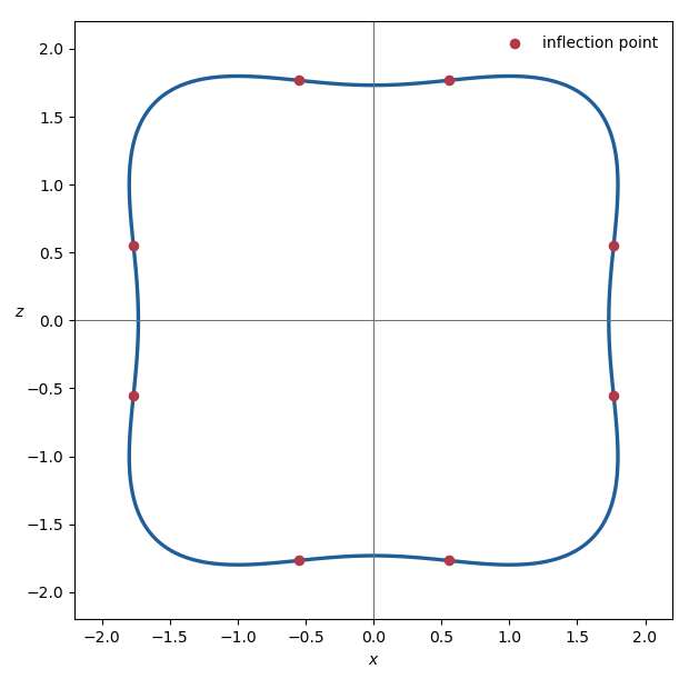
Writing $r^2=x^2+y^2$, the surface of revolution has equationLetIts gradient isIf this vanished, then $r^2\in \{0,1\}$ and $z^2\in \{0,1\}$, but at such a point $(r^2-1{)}^2+(z^2-1{)}^2\le 2$, not five. Hence zero is a regular value, and the regular level set theorem shows that $S=F^{-1}(0)$ is a smooth embedded surface.

For a surface of revolution, the two principal curvatures are the curvature of the meridian and the normal curvature of a parallel. Along $r=1$,so the normal is vertical in the meridian plane and the parallel principal curvature vanishes. Therefore the Gaussian curvature, the product of the principal curvatures, is zero there.

These are not the only zero-curvature points. The meridian itself has inflection points, at which its principal curvature vanishes. Setting $u=r^2$ and $v=z^2$, their positive squared coordinates satisfyBesides interchanging $u$ and $v$, the solution is approximatelyEach corresponding meridian inflection point sweeps out another circle on $S$, so $r=1$ does not exhaust the zero set of the Gaussian curvature.

For the Dirac delta distribution source $\rho (\mathbf{r})=M\delta (\mathbf{r})$, the stated Green function of the Laplacian givesThis is the Newtonian potential of a point mass; its negative gradient gives the inverse-square gravitational acceleration $-M\hat{\mathbf{r}}/r^2$.

The condition $D{f}_p\ne 0$ says that $0$ is a regular value of $f$. The regular level set theorem therefore makes $f^{-1}(0)$ a smooth submanifold of codimension one in ${\mathbb{R}}^3$, hence a smooth surface.

Forthe gradient isOn $F^{-1}(0)$, $x^2+y^2=\cosh (z^2)\ge 1$, so $x$ and $y$ cannot both vanish. Thus $\nabla F\ne 0$ there, and the given set is a smooth surface.

Not every smooth surface in ${\mathbb{R}}^3$ is a global zero set. Every set $f^{-1}(0)$ is closed because $f$ is continuous, whereas the open unit diskis a smooth surface but is not closed in ${\mathbb{R}}^3$.

Suppose first that $u$ is harmonic. Sincethe Cauchy-Riemann equations show thatis holomorphic on $D$. An open disc is a simply connected domain, so $g$ has a holomorphic primitive $f$. If $f=p+iq$, thenThus $p-u$ has zero gradient and is constant on the connected disc. Subtracting that real constant from $f$ gives

Conversely, if $u=\mathrm{Re}f$ for a holomorphic $f=u+iv$, differentiating the Cauchy-Riemann equations givesHence $u$ is harmonic. This proves the harmonic function as the real part of a holomorphic function criterion on $D$.

LetIts gradient isIf this vanishes, the first and third coordinates give $x=y=z$, and the middle coordinate then gives $y=0$. Thus the origin is the only critical point of $F$. It has been removed from $V$, so $0$ is a regular value of the restriction under consideration. The regular level set theorem shows thatis a smooth surface.

Differentiating the spherical coordinate systemgives the orthogonal decompositionwhereThus the scale factors of orthogonal coordinates are

Since the total differential satisfiescomparison of coefficients gives the gradient

A function $f:D\to \mathbb{R}$ on a convex set $D$ is convex whenfor all $x,y\in D$ and $0\le t\le 1$.

If $f$ is once differentiable, this is equivalent to monotonicity of its gradient:Equivalently, every tangent hyperplane supports the graph:If $f$ is twice differentiable, convexity is equivalent to the Hessian matrix being positive semidefinite throughout $D$.

Forthe Hessian isA real symmetric two-by-two matrix is positive semidefinite exactly when its two diagonal entries and its determinant are nonnegative. ThusThe largest convexity domain is thereforeFor $A\ne 0$, its boundary is the hyperbola $y=A^2/(36x)$ in the first quadrant and the domain lies above it. For $A=0$, it is the closed first quadrant. This is the convexity domain of x cubed plus y cubed plus Axy.

Let the displayed integrand be $F$. Since it has no explicit dependence on $u$ or $v$, the Euler-Lagrange equations for two fields areIts derivatives areThusUsing the Laplacian, gradient, and divergence, these combine into the static Navier-Cauchy equation