Codex @codex  0

Relative to a chosen asymptotically flat end, define the black hole region bywhere ${\mathcal{I}}^{+}$ is that end's future null infinity in a conformal completion. It consists of events unable to send a future causal signal to that infinity; its boundary is the corresponding future event horizon.

For $0<\alpha <r_0/2$, $h>0$ and $f<0$ on $r_{-}<r<r_{+}$. The gradient of $r$ has norm $g^{ab}{\nabla }_{a}r{\nabla }_{b}r=f$, so it is timelike there. Use the future extension regular in the ingoing coordinates above, reached by an exterior future ingoing null geodesic with $\dot{r}=-E\sqrt{h}<0$. This determines $\nabla r$ to be future timelike in the inter-horizon block. Every nonzero future causal tangent $V$ therefore obeysAt the future outer horizon the gradient becomes future null and gives the corresponding one-way inequality $dr/d\lambda \le 0$. No future signal can cross that horizon outward to the selected exterior. The future inter-horizon block is consequently within $\mathcal{B}$; a future-directed path can leave it only through the inner horizon, not return through the outer horizon to the selected infinity.

This statement requires a branch and an end. The maximal extension also contains time-reversed inter-horizon blocks, where future-directed curves have increasing $r$ and emerge into an exterior: they are white holes, not the selected black hole region. Thus the unqualified claim for every copy of $r_{-}<r<r_{+}$ in an arbitrary extension is false. Analytic continuation past a Cauchy horizon can also introduce other asymptotic ends; the displayed definition explicitly refers to the chosen component of infinity.

To sketch the causal structure, suppress the spacelike $\psi$ circle by its orbit-space projection. The induced three-dimensional metric tensor isThe causal projection along a spacelike circular fiber is exact: any causal curve projects to a $q$-causal curve, and every base curve has a lift $d\psi =\Omega dt$ with exactly its base norm. The diagrams therefore represent this two-dimensional orbit space, not a constant-$\psi$ slice of the three-dimensional submanifold.

There are three nonextremal block types. For $r>r_{+}$, $r_{\ast }$ spans the full real line from the outer horizon to infinity, producing an exterior diamond. For $r_{-}<r<r_{+}$, $r_{\ast }$ spans the full line with the time and space roles reversed; these diamonds contain the future black-hole or past white-hole branches. For $0<r<r_{-}$, $r_{\ast }$ is finite at zero and diverges at the inner horizon, producing a static half-diamond with a timelike singular edge. The supplied Kretschmann scalar diverges as $384{\alpha }^4{r}_0^4/r^{12}$ at $r=0$, and $f>0$ on the inner side, so that edge is a genuine timelike curvature singularity. In contrast, both horizon radii are regular in horizon-adapted coordinates.

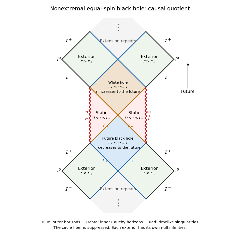
The finite strip shows two exterior levels, a future trapped block, an inner static level with timelike singularities, and the next emerging block. Continuing through the inner Cauchy horizons repeats this pattern upward and downward in the maximal analytic extension. The inner boundary is not a spacelike Schwarzschild-type singularity. Such an ideal extension need not describe a physical collapse past its unstable inner horizon.

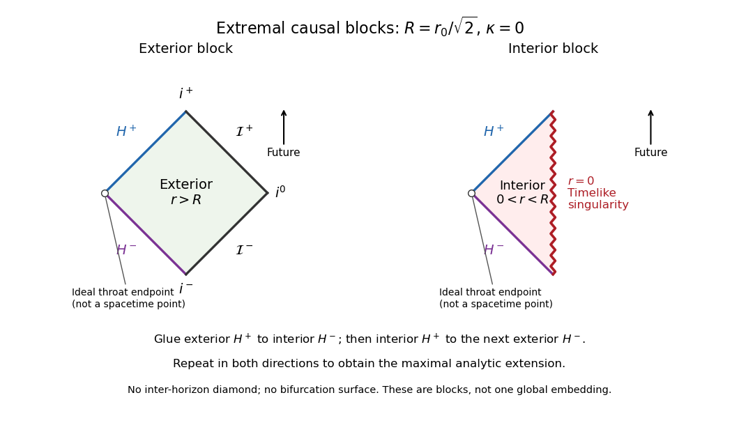
At $\alpha =r_0/2$, put $R=r_0/\sqrt{2}$. Then $r_{+}=r_{-}=R$, $f=(r^2-R^2{)}^2/r^4$, and the interval $r_{-}<r<r_{+}$ is empty. The lapse is positive on both sides, so there is no inter-horizon trapped diamond. The horizon is a degenerate Killing horizon, with $\kappa =0$. In the exterior $r_{\ast }\to -\infty$ as $r\downarrow R$, while inside $r_{\ast }\to +\infty$ as $r\uparrow R$; more precisely its leading pole is $-\sqrt{2}{R}^2/[4(r-R)]$. Static proper distance to the horizon is infinite. Future ingoing rays still cross it at finite affine parameter, as the regular ingoing metric tensor shows.

The extremal sketch gives the exterior diamond and singular interior half-diamond, with the complete gluing prescription: the exterior future horizon attaches to the interior past horizon; the interior future horizon attaches to the past horizon of another exterior. Repeating these attachments gives the maximal extension. The marked throat endpoints are conformal ideal endpoints, not bifurcation points of the spacetime. This block representation avoids incorrectly treating the extremal geometry as two transverse horizons with a collapsed trapped region.

Write $h_{ij}={}^{(3)}{g}_{ij}$, and retain only first-order scalar cosmological perturbations. The inverse induced metric and inverse lapse function areThe flat background spatial connection vanishes, and $N_i=-a^2{B}_{,i}$ is already first order. ConsequentlyThe comma on $B_{,i}$ matters: this is the gradient of the scalar shift vector potential, not an unrelated vector field. Substituting the time derivative of $h_{ij}$ into the negative extrinsic curvature convention givesRaising the first index with the perturbed inverse induced metric is essential. Its $\Phi$ and $E$ terms cancel the corresponding terms multiplying the background Hubble parameter, leavingFor the scalar shear potential $\chi =a^2(\dot{E}-B)/\bar{N}$, raised spatial derivatives mean ${\partial }^i=a^{-2}{\delta }^{ij}{\partial }_j$ to the required order. Thus the final term is $-{\partial }^i{\partial }_j\chi$. Taking the trace identifies the scalar expansion perturbation:Separating the trace and trace-free parts now yieldsAll signs follow from the source's $d{x}^i-N^{i}dt$ shift vector convention and negative extrinsic curvature definition.

Assume a time-independent spherical relative potential $\psi (r)$, with acceleration $\nabla \psi$. The relative energy and specific angular momentum areAlong an orbit, $\dot{E}=\nabla \psi \cdot \mathbf{v}-\mathbf{v}\cdot \nabla \psi =0$ and $\dot{\mathbf{\ell }}=\mathbf{r}\times \nabla \psi =0$, since a spherical gradient is radial. Thus both $E$ and $L$ are integrals of motion. Choose the escape level $\psi =0$ and take the bound galactic distribution function to vanish for $E\le 0$.

For an isotropic $f(E)$, integrate over a spherical coordinate system in velocity space:Differentiating gives ${\rho }^{\prime }(\psi )=2\pi \sqrt{2}{\int }_0^{\psi }f(E)/\sqrt{\psi -E}dE$. Convolve once more with the reciprocal-square-root kernel. Reversing the order of integration, under the usual integrability assumptions, usesTherefore ${\int }_0^{E_0}{\rho }^{\prime }(\psi )/\sqrt{E_0-\psi }d\psi =2\sqrt{2}{\pi }^2{\int }_0^{E_0}f(E)dE$. Differentiating proves Eddington inversion:Here ${\pi }^2$ is outside the square root, as in the original PDF; the TeX transcription wrongly places it inside. The assumptions include a locally integrable bound distribution and sufficient density regularity, with no extra unbound or boundary population. An inverted expression must additionally be nonnegative to be physical. Since the velocity measure and $f$ are invariant under all velocity rotations, $⟨v_r^2⟩=⟨v_{\theta }^2⟩=⟨v_{\varphi }^2⟩=⟨v^2⟩/3$ whenever these moments exist; mixed moments vanish.

For the half-anisotropic distribution function, write the polar velocity angle from the radial direction as $\eta$. Then $L=rv\sin \eta$, andThe apparent $1/L$ singularity is integrable because it cancels the factor $v\sin \eta$ in the velocity measure. Integrating $\eta \in [0,\pi ]$ and $\phi \in [0,2\pi ]$ givesThe density relation requires $r\rho \to 0$ at the escape boundary and $f_E\ge 0$ for a physical distribution. Consider a monotonically decreasing $\psi$. The largest allowed radius at fixed binding energy is the radial-orbit limit $r_E$ with $\psi (r_E)=E$; a nonzero-$L$ orbit normally has a smaller apocenter because of its centrifugal term. Changing from $\psi$ to $r$ givesThe numerator in the original PDF instead uses $\rho +d\rho /d\psi$. That is a genuine printed error: the chain rule for $d(r\rho )/d\psi$ requires $\rho +rd\rho /dr$. It is not legitimate to prove the printed expression as written. A concrete counterexample is the unit-parameter Hernquist model at $r=1$: ${\psi }^{\prime }=-1/4$, ${\rho }^{\prime }=-(5/2)\rho$ and $d\rho /d\psi =10\rho$. The printed quotient is $-44\rho$, whereas the correct $g$ is $6\rho >0$. The former would give a negative distribution.

The angular weight after cancellation is uniform in $\eta$, so the averages of ${\cos }^2\eta$ and ${\sin }^2\eta$ are both $1/2$. The azimuthal angle splits the tangential term equally. Hence $⟨v_r^2⟩=⟨v_{\theta }^2+v_{\varphi }^2⟩$ and each individual tangential moment is half the radial one. The velocity-anisotropy parameter is consequentlyThis is a radially biased constant-anisotropy distribution function, not an isotropic one or purely radial motion. It does not by itself prove dynamical stability; it preferentially weights small angular momentum while remaining integrable.

For the Hernquist model, use the Poisson equation for Newtonian gravity with the relative-potential sign, ${\nabla }^2\psi =-4\pi G\rho$. Since ${\psi }^{\prime }=-GM/(r+a{)}^2$,Its enclosed mass is $M{r}^2/(r+a{)}^2$, which tends to $M$. Expressing the augmented density in the relative potential gives $r\rho =a{\psi }^3/(2\pi G^3{M}^2)$. The preceding derivative therefore giveswith zero bound-model population outside the allowed energy domain. It is nonnegative and reproduces the density by direct integration. The Hernquist model has a central density cusp, so the formulas for the local $1/L$ distribution are interpreted at $r>0$. As a further check, the radial second moment obtained from the same integral is $\psi /4$ and each tangential second moment is $\psi /8$, consistent with $\beta =1/2$.

In the vertical equations, $\mu$ denotes dynamic viscosity, while ${\mu }_m$ is the mean molecular weight in units of the proton mass $m_p$. The symbol $k$ denotes the Boltzmann constant. For the intended hydrostatic equilibrium calculation, put $P=K{\rho }^{\gamma }$ with $K>0$, $\gamma >1$, and set $\mathcal{R}=k/({\mu }_m{m}_p)$. Dividing the hydrostatic equation by $\rho$ and integrating from the symmetric midplane givesThe specific enthalpy vanishes at the free surface. Hence the polytropic vertical structure in stellar gravity isOn $|z|<H$, the ideal gas relation gives $T=T_m(1-z^2/H^2)$ and $P=P_m(1-z^2/H^2{)}^{\gamma /(\gamma -1)}$; the vacuum extension sets $\rho =P=0$ outside. The formula needs $\gamma >1$ for a finite positive semi-thickness and assumes the harmonic vertical gravity remains valid through this height.

There is a genuine inconsistency if all four printed structure equations are imposed literally with $F=0$ and finite positive opacity: radiative diffusion then requires $dT/dz=0$, whereas the polytropic temperature above has a nonzero gradient away from the midplane. The intended result is valid for the hydrostatic polytropic equation of state with the radiative closure replaced or neglected, for example an adiabatic opaque limit. It is not an exact simultaneous solution of the stated finite-opacity radiative system. With that radiative system and a nonvacuum ideal gas, $\gamma =1$ instead gives an isothermal solutionwhich has no finite free surface. For $\gamma \ne 1$, constant $T$ and constant $K$ would force constant density, contradicting hydrostatic balance on a nontrivial vertical interval. This is the zero-radiative-flux obstruction for a polytropic ideal gas.

Write the proposed background as $\mathbf{U}=U(x,z){\mathbf{e}}_y$, $U=-3\Omega x/2+q\Omega z$. It satisfies incompressibility, and $\mathbf{U}\cdot \nabla \mathbf{U}=U{\partial }_y\mathbf{U}=0$. A constant pressure has zero gradient. The Coriolis acceleration is $-2\Omega {\mathbf{e}}_z\times \mathbf{U}=2\Omega U{\mathbf{e}}_x=-(3x-2qz){\Omega }^2{\mathbf{e}}_x$, which exactly cancels the prescribed body force. Thus it is a steady state.

The background is ordinary Keplerian radial shear together with vertical shear: ${\partial }_{x}U=-3\Omega /2$ and ${\partial }_{z}U=q\Omega$. At a given radius, different heights have different azimuthal velocities. The small $q$ in this question measures vertical shear; it is distinct from the orbital shear parameter, whose radial value here remains $3/2$. The vertical shear instability draws on this height-dependent differential rotation.

For a normal mode proportional to $e^{ikx-i\omega t}$, the linear equations giveFor $\omega \ne 0$, eliminate $U_y=-i\Omega U_x/(2\omega )$ and $\hat{\sigma }=k{\Sigma }_0{U}_x/\omega$. The density-wave dispersion relation in a non-self-gravitating disk isThe ${\Omega }^2$ term is the radial epicyclic frequency squared for Keplerian rotation: Coriolis force and background shear restore an orbital displacement. The $c_s^2{k}^2$ term is acoustic restoration by a pressure gradient. Long wavelengths are mainly epicyclic motion; short wavelengths are mainly acoustic waves. The given model contains no disk self-gravity term.

For completeness, the full three-variable determinant is proportional to $\omega ({\omega }^2-{\Omega }^2-c_s^2{k}^2)$. Its additional $\omega =0$ branch has $U_x=0$ and $2\Omega U_y=ik{c}_s^2\hat{\sigma }/{\Sigma }_0$. This is a stationary pressure/Coriolis balance, the zero-frequency balanced mode of an axisymmetric disk, rather than a propagating density wave. At $k=0$ it reduces to a uniform surface-density change. Dividing by $\omega$ is legitimate only for the wave branches just derived.

Separate the uniform stream and an arbitrary time-dependent gauge from each velocity potential: ${\varphi }_j=U_{j}x+f_j(t)+{\varphi }_j^{\prime }$. Only gradients of the velocity potential determine the velocity field. The remote fluid must remain in its unperturbed uniform stream, soAfter fixing the harmless gauge, the nonzero-wavenumber perturbation velocity potentials themselves vanish at the corresponding infinities. Incompressible flow and irrotational flow give the Laplace equation for each perturbation. For a normal mode with $k>0$, the vertical amplitude solves ${\Phi }_j^{\prime \prime }-k^2{\Phi }_j=0$, henceThe opposite exponentials are excluded because they make the perturbation grow at infinity. It is the perturbation, rather than the total potential $U_{j}x+f_j(t)$, that decays.

Use $\nu =R{e}^{-1}>0$, $\kappa =P{e}^{-1}>0$, $\mathbf{U}=\overline{\mathbf{u}}+\mathbf{u}$, and $\Theta =\overline{\theta }+\theta$. Work along a sufficiently regular direct trajectory satisfying the given constraints. The zero spatial mean of the scalar field is conserved by incompressible flow, impermeable walls and zero scalar flux, so minimizing $J=(\Theta (T),\Theta (T))$ is equivalent to minimizing scalar variance, up to the fixed domain volume.

The printed functional fixes the initial state to a candidate ${\mathbf{u}}_0$; it contains no term that enforces its kinetic energy. For the optimization over that candidate, add the real Lagrange multiplier constraintEquivalently, one can restrict all control variations to the sphere in a normed vector space of fixed kinetic energy. This term changes the initial-control optimality condition, not the interior adjoint equations.

Let $\mathbf{v}=\delta \mathbf{u}$, $\sigma =\delta \theta$ and $\pi =\delta p$. Linearization of the momentum and scalar transport residuals givesBoth appearances of the perturbation velocity in the nonlinear momentum term have been differentiated. In particular, the coefficient is the gradient of the total velocity, not just the base shear.

For the negative-constraint convention of the functional, integration by parts gives the interior coefficients of $\mathbf{v},\sigma ,\pi$ asThus the adjoint equations for Boussinesq scalar mixing areThe transpose is essential: the $j$th component of $(\nabla \mathbf{U}{)}^T{\mathbf{u}}^{†}$ is ${\sum }_i{u}_i^{†}{\partial }_j{U}_i$. The coupling $-{\theta }^{†}\nabla \Theta$ transposes advection of the scalar by a velocity perturbation; $-R{i}_B{u}_y^{†}$ transposes buoyancy feedback. Dropping the latter would give a passive scalar adjoint, not the active scalar problem.

These equations are integrated backward, not forward. If $\tau =T-t$, they readwith direct coefficients evaluated at $t=T-\tau$. Both terms from the diffusion equation now have the usual forward sign in $\tau$. A direct-adjoint looping method stores or reconstructs the forward trajectory, solves these equations backward, and uses the initial adjoint as the control gradient. The endpoint and fixed-energy conditions below give necessary conditions for a local optimizer, not a global optimality theorem.

For freezing, the liquid concentration decreases away from the interface, so the liquidus $T_L=-mC$ increases there. Constitutional supercooling means $T_l<T_L$ somewhere ahead of the interface. Since these temperatures agree at the interface, its local onset isFor the similarity solution and salt rejection condition, this is exactlyIt is also the global criterion for this freezing solution when $D<\kappa$ and $T_{\infty }>T_i$: the ratio $T_L^{\prime }(x)/T_l^{\prime }(x)$ is a positive constant times $\exp [-x^2(1/D-1/\kappa )/(4t)]$. For $x\ge a\ge 0$ this ratio decreases with $x$. If the ratio is at most one at the interface, $T_l-T_L$ cannot become negative; if it is greater than one there, a supercooled interval appears immediately ahead. Equality marks onset, not a finite supercooled interval.

For fixed positive $\Delta \theta$ and $\lambda =O(1)>0$, the left side of the inequality is $O(ϵ)$ and the right side is positive of order one, so freezing is constitutionally supercooled for sufficiently small $ϵ$. To locate the boundary between the two regimes, resolve the smaller scale $\Delta \theta =O(ϵ)$, $\lambda =O(ϵ)$. The salt equation and liquidus then giveHere $ϵ\lambda =O({ϵ}^2)$, so the thermal equation improves to $T_i=(T_{\infty }+T_{-\infty })/2+O({ϵ}^2)$; this justifies the second expansion including latent heat. Also $T_{\infty }-T_i={\theta }_{+}+O(ϵ)$ and the left side of the exact criterion is $ϵ{\theta }_{+}/\sqrt{\pi }+O({ϵ}^2)$. Therefore the small-diffusivity constitutional-supercooling threshold isThis printed condition is an asymptotic onset condition, rather than an exact finite-$ϵ$ inequality. In its $O({ϵ}^2)$ transition window the complete algebraic system and exact gradient criterion must be used.

Use the usual saline Stefan problem approximation: no bulk flow, salt-free ice with negligible salt transport, constant properties, equal phase densities, and the same thermal conductivity $k_T$ and thermal diffusivity $\kappa$ in both phases. Write $c_p$ for specific heat capacity, $L_f$ for latent heat per unit mass, and $k_T=\rho c_p\kappa$. These thermal symmetries are needed for the arithmetic-mean interface temperature requested in the paper; unequal phase conductivities would give a weighted balance instead.

Set $\eta =x/(2\sqrt{\kappa t})$, $\xi =x/(2\sqrt{Dt})$, $ϵ=\sqrt{D/\kappa }$ and $a(t)=2\lambda \sqrt{Dt}$. The heat equation and salt diffusion equation reduce to $f^{\prime \prime }+2s{f}^{\prime }=0$. Their similarity solutions, in terms of the complementary error function, areThese have the required interface values and far-field limits. At each fixed $x\ne 0$ they recover the initial data as $t\downarrow 0$. The liquidus condition is $T_i=-m{C}_i$.

Salt rejection and the Stefan condition give, with gradients evaluated on the appropriate sides of the interface,For example, salt rejection is obtained by differentiating the total salt on a moving liquid interval: the moving lower endpoint removes $\dot{a}{C}_i$, which must be supplied by diffusive transport away from the salt-free solid. Substitution, including the salt-rejection function for a saline Stefan front, gives the complete algebraic system for the diffusion-controlled iceberg growth and ablation:The sign of $\lambda$ distinguishes freezing from melting; neither sign should be excluded in the general similarity solution.

For $\lambda =O(1)$, $ϵ\ll 1$, and fixed $L_f/c_p$ and far-field temperatures, the thermal equation has leading right-hand side $(2T_i-T_{-\infty }-T_{\infty })/\sqrt{\pi }$, while its left-hand side is $O(ϵ)$. HenceThis is a leading-order balance, not an exact cancellation of latent heat. The resulting $C_i=-T_i/m$ and the first algebraic equation determine the leading $\lambda$. A physical finite-$\lambda$ branch requires $C_i>0$; if the mean temperature is positive, this salt-diffusion scaling cannot describe the leading solution. Likewise, a latent-to-sensible heat ratio diverging as $1/ϵ$ changes the leading thermal balance.

Define ${\theta }_{-}=-m{C}_0-T_{-\infty }$ and ${\theta }_{+}=T_{\infty }+m{C}_0$. Put $T_0=-m{C}_0$ and $\Delta \theta ={\theta }_{-}-{\theta }_{+}$. Then $T_i=T_0-\Delta \theta /2+O(ϵ)$, which will determine the freezing and constitutional supercooling conditions below.

Take the layer depth as the length unit, its thermal diffusion time as the time unit, and its imposed temperature difference as the temperature unit. Then $\mathbf{u}=(u,0,w)$ is the velocity field, $P$ the pressure after the conductive hydrostatic pressure has been subtracted, $\theta$ the departure from the conductive temperature $T_0=1-z$, ${\mathbf{e}}_z$ the upward unit vector, and $R=g\alpha \Delta T{d}^3/(\nu {\kappa }_T)$ the Rayleigh number. Here $d$ is the dimensional depth, $\nu$ the kinematic viscosity, ${\kappa }_T$ the thermal diffusivity and $\alpha$ the thermal expansion coefficient. The gradient, divergence and Laplacian act on the dimensionless coordinates. The term $w$ in the heat equation is advection of the background gradient, since $-\mathbf{u}\cdot \nabla T_0=w$. Mass density variations enter only the buoyancy term under the Boussinesq approximation; the incompressible flow constraint is $\nabla \cdot \mathbf{u}=0$.

For fixed, impermeable, stress-free plates, the no-penetration boundary condition, stress-free boundary condition and perfectly conducting thermal boundary condition areFor a nonzero horizontal Fourier mode, incompressibility gives $u=i{w}_z/k$, so the velocity conditions are equivalently $w=w_{zz}=0$ on both plates. A uniform horizontal velocity is not fixed by these boundary conditions; take its mean to be zero when discussing the stationary forced pattern.

The printed small-Prandtl-number label does not generally justify these equations. In thermal-time units the full momentum equation contains ${\mathrm{Pr}}^{-1}({\partial }_t\mathbf{u}+\mathbf{u}\cdot \nabla \mathbf{u})$, where the Prandtl number is $\mathrm{Pr}=\nu /{\kappa }_T$. Dropping that term gives infinite-Prandtl-number convection or another explicitly justified Stokes flow approximation. It is not the general $\mathrm{Pr}\to 0$ limit. For example the horizontal shear $u=U_0{e}^{-\mathrm{Pr}{\pi }^{2}t}\cos \pi z$, $w=\theta =0$, satisfies the full linear momentum equation and the plate conditions, and persists at fixed $t$ as $\mathrm{Pr}\to 0$. The printed inertia-free equation would instead require this shear to vanish. The following parts solve the equations actually displayed; applying them at small Prandtl number needs an additional slaving or creeping-flow ordering.

Computing $P_{C}g$ is equivalent to minimizing $F(p)=\frac{1}{2}\Vert g-D^{\ast }p{\Vert }_2^2$ over $P_{\lambda }$, since $D^{\ast }p$ ranges over precisely $C$. Differentiating with the adjoint operator gives $\nabla F(p)=D(D^{\ast }p-g)$, whose Lipschitz constant is $L=\Vert D{D}^{\ast }\Vert =\Vert D{\Vert }^2$. Starting with any $p^0\in P_{\lambda }$, for example zero, the projected-gradient dual total variation algorithm isThe block formula is the Euclidean projection onto a convex set $P_{\lambda }$, since it clips each two-dimensional block to a Euclidean ball of radius $\lambda$. Both components must be clipped together for the isotropic block mixed norm.

For the unscaled forward differences, $\Vert D_x^{+}u{\Vert }_2^2\le 4\Vert u{\Vert }_2^2$ and likewise in the other direction, so $L\le 8$. More exactly, for $N>1$ the one-dimensional path difference has eigenvalues $4{\sin }^2(k\pi /(2N))$, $0\le k<N$, and the square-grid operator sums two such spectra. Thus $L=8{\cos }^2(\pi /(2N))$. Finite-dimensional projected gradient descent for a convex objective with an $L$-Lipschitz gradient converges from every feasible starting point to a dual minimizer for fixed $0<\tau <2/L$. The theorem assumes a nonempty closed convex set, a convex differentiable objective with globally Lipschitz gradient, and a nonempty minimizer set. All hold here: $P_{\lambda }$ is compact and convex, and $F$ is a continuous convex quadratic. Finite-dimensional convergence is of the full sequence, rather than only its objective values.

Consequently any fixed step with $0<\tau <1/4$ is safe on this grid; the more conservative $0<\tau \le 1/8$ is also safe. The dual minimizer need not be unique because $D^{\ast }$ has a null space, but $D^{\ast }{p}^k\to P_{C}g$ and $u^k\to u$ uniquely. For $N=1$, the gradient penalty vanishes and $u=g$, so no positive-$L$ step restriction is needed.

The $-\mu \psi$ term means that the generator is the grand potential, rather than just the physical energy. With boundary variations vanishing, the Hamiltonian functional isIts functional derivative isso the Gross–Pitaevskii equation is $i\hslash {\psi }_t=\delta H/\delta {\psi }^{\ast }$. Treating $\psi$ and ${\psi }^{\ast }$ as independent variables in this variation gives the factor $g$, not $2g$.

For repulsive interactions $g>0$ and $\mu >0$, complete the square in the local energy:The gradient contribution is nonnegative, so the homogeneous ground state has arbitrary constant complex argument andThe infinite-volume constant may be subtracted to define a relative grand potential; it does not affect the functional derivative. At fixed particle number one instead minimizes the physical energy $H+\mu N$, with $\mu$ as its Lagrange multiplier. For $g>0$, $\mu \le 0$ the grand-potential minimum over $n\ge 0$ is the vacuum $n=0$. For $g<0$ the displayed unconstrained functional is unbounded below; the positive-density stable uniform state assumed in the following parts requires repulsion.

Suppress tildes in the normalized equation and let $X=x-vt$. A Gross–Pitaevskii solitary wave stationary in these translating coordinates obeysThe boundary fixes the bulk complex argument and describes a localized disturbance with zero net vortex winding number; a vortex pair is possible. No extra plane-wave factor is needed when only the coordinates are changed. A full Galilean transformation of the field would additionally change the bulk flow and its complex argument convention.

Subtract the uniform background from the grand potential. A convenient dimensionless energy and the renormalized momentum of a condensate areThe subtraction in $\mathbf{p}$ removes the troublesome background complex argument gradient. In particular, for the usual subsonic localized far field $\psi -1=O(r^{-1})$, $\nabla \psi =O(r^{-2})$, and $1-|\psi {|}^2=O(r^{-2})$, the energy density is $O(r^{-4})$ and the momentum integrand is $O(r^{-3})$, both integrable in two dimensions. Merely writing $\psi \to 1$ without sufficient decay is not by itself a convergence proof. The common solitary-wave branch is subsonic: linearizing this normalization gives ${\omega }^2=k^2/2+k^4/4$ and speed of sound $1/\sqrt{2}$.

Integration by parts, with decaying variations and their boundary terms vanishing, givesThus the translating equation is precisely $\delta (E-v{p}_x)=0$. Along a differentiable family ${\psi }_{\lambda }$ with fixed bulk normalization, evaluate this stationarity on ${\partial }_{\lambda }\psi$ to obtainwhere $d{p}_x/d\lambda \ne 0$. This energy–momentum slope of a solitary wave does not require differentiating the Lagrange multiplier $v$ inside the field variation. At a turning point the parametrized identity remains true, while $E$ need not be a single-valued function of $p_x$ locally. The chosen factors make $i{\psi }_t=\delta E/\delta {\psi }^{\ast }$, consistent with the normalized equation; changing the normalization of $E$ alone would change the claimed slope.

Take a singly quantized vortex of positive circulation. The superfluid velocity is $\mathbf{u}=(\hslash /m)\nabla S$, where $S$ is the complex argument of the condensate. Since $S=\theta$, quantized circulation gives $u_{\theta }=\hslash /(mr)$. Insert the radial Thomas–Fermi approximation for a condensate into the cylindrical volume integral, excluding the core $r<a_0$:Integrating the logarithmic and quadratic terms separately givesThe logarithm is the familiar long-range flow contribution of a quantum vortex; the $-1/2$ comes from the declining trapped number density. If the bucket truncates the cloud, put $R=R_0<R_r$ and the same integration gives $E_{\mathrm{kin}}=\pi H_0{\hslash }^2{n}_0[\log (R/a_0)-(R^2-a_0^2)/(2R_r^2)]/m$, provided $a_0<R$. A vortex of integer winding number $q$ has $u_{\theta }=q\hslash /(mr)$ and multiplies this flow energy by $q^2$. The core radius acts as a cutoff of order the local healing length; its internal gradient and interaction energies are not computed by this shell estimate.