
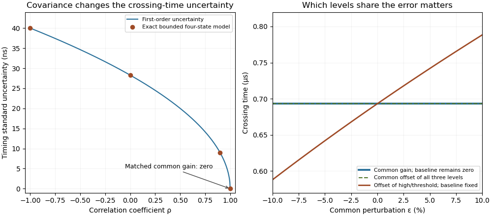
Covariance changes RC timing uncertainty, while gain and offset cancellation depend on the full measurement model
. Original calculation for a 1 V high level, 0.5 V threshold and 1 µs time constant. Exact four-state bounded-error checks are compared with first-order propagation. The right panel distinguishes common gain, a two-level offset with fixed baseline, and a common offset of all three levels. Its common perturbation sets gain or offset . No measured uncertainty data are used. Details.
A raw laser pulse energy estimate and its baseline correction can contain the same readout error. Let be the raw gate integral, the estimated integrated background and the corrected result. Linearity of covariance gives the exact identityFor this linear measurement model, the law of propagation of uncertainty is exact whenever the input variances exist. Its general form includes the sensitivity coefficients and covariance terms.[ref]
Guidelines for Evaluating and Expressing the Uncertainty of NIST Measurement Results by Barry N. Taylor and Chris E. Kuyatt. Appendix A, equation A-3
Positive covariance reduces the variance of this difference; it would instead increase the variance of a sum.An original shared-offset model makes the mechanism explicit. For fixed gate duration , writewhere is a common additive power-readout offset with standard uncertainty , while and are independent zero-mean energy errors, independent also of . Then , and shared-offset cancellation in a baseline-corrected pulse integral gives . The shared offset contributes no uncertainty to this difference. It need not be small or separately known.
Choose , , and . The shared energy contribution is in each reading. Thus , and , yielding . Incorrectly discarding the covariance gives .
Cancellation weakens if the offset changes between acquisitions. Replace by two offsets with the same standard uncertainty and correlation coefficient . Under the same independent residual-error assumptions,At , the chosen example gives . A baseline taken far away in time cannot simply be assigned the covariance of an unchanged offset.
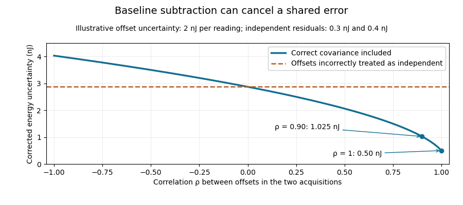
Shared baseline errors cancel according to their correlation
. Original numerical model with a 2 nJ offset uncertainty in each acquisition and independent residual uncertainties of 0.3 nJ and 0.4 nJ. The comparison curve incorrectly treats the shared offsets as independent. Details.
A sampled implementation has the same structure. If a vector of readings has covariance matrix , and fixed integration weights give and , thenA constant offset cancels when the weights sum to the same gate duration: . This does not justify using pulse-contaminated readings as background. Matched blank sequences, collected with the actual timing, help characterize the needed noise correlations.
The historical NIST TC-24 apparatus used a thermocouple-based absorbing plate and averaged baseline measurements before and after laser injection to compensate background and thermal drift.[ref]
Calibration Service for Low-level Pulsed-Laser Radiometers at 1.06 µm: Pulse Energy and Peak Power by Rodney W. Leonhardt. §3.5, printed p. 8; §7.2, Leakage Effect
The offset model above is an independent illustration, not a reconstruction of that instrument's uncertainty budget.Covariance-consistent rescaling of whitened spectral coordinates changes measurement units or mixes coordinates while transforming their noise model at the same time. If an invertible matrix maps a spectral vector to , thenThe covariance follows directly from the expectation of the transformed error outer product. For positive-definite ,Thus the inverse-covariance inner product, its norms and the resulting whitened angle are invariant. Invariance of noise-whitened spectral angles to the whitening factor establishes the related freedom to rotate the fully whitened coordinates.
For an original example, let , and . Their noise-whitened angle has cosine , or angle about . Converting only the first raw coordinate's numerical units by a factor of 1000 gives and . Using that transformed covariance keeps the cosine exactly .
If the shapes are rescaled but the old covariance is mistakenly retained, the calculated cosine becomes approximately , suggesting an angle only about . A unit conversion would then appear to destroy the separation between signal and nuisance. That apparent change comes from inconsistent uncertainty accounting.
For any full whitening factor , the transformed factor satisfies and gives . The pinned SciPy documentation describes whitening and demonstrates a near-identity covariance after transformation.[ref] Measurement propagation likewise retains all covariance terms under a linear transformation.[ref]
The invertibility condition matters. Noninvertible spectral compression versus a coordinate change can discard information and need not preserve these angles. A transformation estimated from the same noisy observations also brings estimation uncertainty beyond the fixed-matrix identity proved here.
The covariance of count-conserving rebinned Raman channels records the shared noise created when one measured channel contributes to several output channels. For a fixed deterministic rebinning matrix and an input count vector with covariance matrix , the output is andThis identity needs finite second moments, not a Gaussian approximation. Raman spectral rebinning with conserved integrated counts describes the count-preserving map; retaining its full covariance matrix is necessary for uncertainties of sums and fitted spectral features.[ref]
Consider independent input counts with means and and Poisson distribution variances equal to those means. Split them deterministically usingThe three output means are . Their total has variance , exactly the original total variance, and standard deviation . Keeping only diagonal entries would give variance and standard deviation about , understating the uncertainty of the conserved total.
The rank deficiency from deterministic spectral upsampling is visible without matrix inversion: the vector has zero output contrast for every possible input. Three displayed channels therefore contain at most two independent degrees of freedom in this model. Fractional redistribution creates correlated numerical channels; it is different from physically assigning each detected photon randomly to one new channel.
The primary stimulated-Raman apparatus records spectra with array detectors and calibrates their spectral coordinates.[ref]
Femtosecond Broadband Stimulated Raman: A New Approach for High-Performance Vibrational Spectroscopy by David W. McCamant and others. Instrumentation, array detection and frequency-shift calibration; Data Collection, equation 4
When those data are placed on a new spectral grid, the original detector counts remain the source of statistical information. Additional interpolation points do not supply independent photon measurements.The covariance of differential spectral-calibration gains describes the joint errors of gain differences used in several spectral ratios. Let the calibration-error vector be with covariance , and form differences . ThenThis covariance identity is exact for the linear differences; no normal-distribution assumption is required. The first-order relation between gain differences and isotope stiffness ratios is given in separate spectral-calibration gains in isotope stiffness inference.[ref]
Guidelines for Evaluating and Expressing the Uncertainty of NIST Measurement Results by Barry N. Taylor and Chris E. Kuyatt. Appendix A, equation A-3, sensitivity and covariance propagation
For an original shared-reference model, take three gain errors , where is a common scale error and the are independent residual errors with variances . Two sample spectra are compared with the same reference spectrum:The common scale cancels, but the residual reference error remains in both differences:Cancellation of one common influence therefore does not establish independent comparisons.
Choose all three residual standard uncertainties as . Then , with correlation between the differences. Even a much larger common scale uncertainty cancels in this stipulated model. Each inferred log stiffness ratio has error approximately twice its gain difference. Averaging the two log-ratio estimates gives variance and standard uncertainty about . Incorrectly treating them as independent would give only .
This shared-reference floor in averaged isotope stiffness ratios matters when many sample spectra reuse one calibrated reference. Independent extra sample readings reduce their own errors, while a reference component shared by all comparisons remains. Assess covariance from the actual reference reuse, calibration drift and repeated acquisition protocol. The matrix calculation concerns multiplicative calibration errors; uncertain peak assignment, isotope composition and additive spectral offsets need their own contributions.
Coverage excess from central quantiles at a zero-duration atom is the additional distributional probability included when a closed quantile interval captures an entire point mass at zero. Here coverage means probability under the stated duration model. For with , the zero mass is and the positive part is continuous. Let , , and use the lower quantiles from quantiles of a clipped Gaussian acquisition duration.
For the closed central interval , its probability isTo verify this, write the probability as . When both endpoints are positive, the lower left limit is and the upper value is . Once the lower endpoint is zero, its left limit is zero; if the upper endpoint is zero too, the interval contains exactly the zero atom. Endpoint inclusion is therefore part of the probability calculation.
For a nominal 95 percent central construction, zero masses , and give actual probabilities , and respectively. In the middle case, the excess is , not the whole atom: the interval already includes the probability between zero and the upper quantile.
As an original dimensional example, set , and , giving . The nominal central 95 percent interval is approximately and contains probability . SciPy documents the normal cdf and inverse-cdf ppf used to evaluate these Gaussian-component values.[ref]
SciPy 1.16.2 documentation. scipy.stats.norm, Methods: cdf and ppf
A one-sided upper interval or a separately specified probability construction can target a different included probability. Randomized endpoint inclusion at a zero-duration atom would require an explicit randomization rule, not a change made silently after seeing an endpoint equal zero. NIST explains why interval interpretation requires the input distributions and the chosen construction.[ref]
Guidelines for Evaluating and Expressing the Uncertainty of NIST Measurement Results by Barry N. Taylor and Chris E. Kuyatt. §6.3, Expanded Uncertainty
Distributional probability for this conditional acquisition model is separate from a worst-case optical-energy guarantee or a confidence procedure for an unknown fixed parameter. Coverage factor 2026-11-05
A coverage factor multiplies combined standard uncertainty to give expanded uncertainty, . It is dimensionless. Choosing it requires a target coverage and assumptions about the result's distribution and the reliability of the estimated standard deviation.
For a normal distribution with known standard deviation, gives a central interval of about 95 percent probability. With a small sample and an estimated variance, an appropriate Student's t-distribution quantile can be larger. A stated factor therefore communicates a method, not merely an error-bar width.[ref]
Coverage failure under random variance-ratio limits can persist even when the centre is exactly normal, the variance estimate is conservative in expectation, and its absolute error tends to zero. What fails is relative-scale concentration. Let and a positive random scale be independent, and defineThe variance ratio is at every sample size. Its nondegenerate distribution need not approach the constant required in asymptotic conservative Wald coverage under variance-ratio convergence.
Conditional on , a normal critical value gives interval coverage . Therefore unconditional coverage is under the independence assumption. A useful shape calculation isThe function is strictly concave. If , Jensen's inequality puts , with strict inequality for a nonconstant scale. An expectation equality therefore does not reproduce the normal interval's nominal coverage.
For an original strictly conservative example, let take and with equal probabilities. Then , but at nominal 95 percent the exact coverage isThis value is unchanged as grows. Meanwhile tends to zero, showing why absolute consistency at a vanishing variance scale is insufficient. The normal cdf evaluation uses the pinned primary numerical definition.[ref]
SciPy 1.16.2 documentation. scipy.stats.norm, cdf and ppf
If the scale depends on the standardized error, the conditional normal formula above cannot simply be retained; the joint law is needed. NIST likewise distinguishes a justified coverage probability from selecting a conventional uncertainty multiplier.[ref]
A coverage-preserving detector-width bound from a variance interval transforms uncertainty in a nonnegative response variance without imposing a symmetric width error bar. Let and let a random interval have stated frequentist coverage for . Define the width confidence set byFor the true width ,The events are identical, so their coverage probabilities are identical. The transformation does not create coverage that the original interval lacked. Resolution-limit conditioning in finite-input detector calibration explains why working with the variance difference first is useful near a barely resolved detector response.
For an original explicit measurement model, suppose has a normal distribution with mean and known standard deviation . A reading gives an approximately 95 percent interval . Intersecting with the physical range and taking square roots gives . This is an assumed normal model for measuring , not a claim that any difference of fitted squared widths is automatically normal.
If the entire variance interval is negative, the result is an empty physical confidence set for a detector variance difference. Do not replace its negative upper endpoint by zero and report an apparently exact zero width: that changes the confidence-set construction. An empty realization signals disagreement between that interval and the physical parameter range; it can occur even in a valid procedure on an occasional sample that misses the true value.
NIST distinguishes a standard uncertainty from an interval with a justified confidence level and explains the distributional assumptions behind a coverage factor near two.[ref]
Guidelines for Evaluating and Expressing the Uncertainty of NIST Measurement Results by Barry N. Taylor and Chris E. Kuyatt. §§6.2–6.3, Expanded Uncertainty
The normal interval above needs its stated model; the monotone transformation proof itself does not. Application to a detector additionally requires the nonnegative-profile convolution assumptions of finite-input correction in pulse-detector calibration; a correct statistical transformation cannot repair an invalid physical variance identity.Effective repetition count across independent calibration blocks accounts for dependence confined to each acquisition block rather than shared by every stored trace. Suppose block contains empty-interval indicator random variables, all with common probability and within-block correlation coefficient . Assume different blocks are independent. With , summing within-block covariances givesMatching this to the variance of an average of independent indicators yieldsFor equal blocks of size , this reduces to . The denominator involves the block size, not the total ; the single-block expression in effective repetition count for detector intervals with shared drift must not be applied as though the same drift state affected every block.
For an original comparison, fix and . One block gives . Six independent blocks of twenty give . Six very uneven blocks of sizes instead giveAll three designs store the same number of traces. The difference comes from how often the same fluctuating condition is reused. For fixed , , and positive , minimizing favors balanced blocks; this motivates optimal allocation of detector repetitions across calibration blocks when block-preparation costs also matter.
Independence must come from the physical acquisition model. Starting another file does not erase a shared clock, reference calibration, or slowly varying environmental influence. NIST's uncertainty law retains shared-input covariance explicitly.[ref]
Guidelines for Evaluating and Expressing the Uncertainty of NIST Measurement Results by Barry N. Taylor and Chris E. Kuyatt. Appendix A, equation A-3
If drift persists between nominal blocks, those cross-block terms must be added and the displayed formula changes. A cluster bootstrap likewise requires blocks that are suitable independent resampling units.An empty physical confidence set for a detector variance difference occurs when the entire reported interval for the inferred response variance lies below its admissible range. In the nonnegative-profile detector model, . An interval gives a physical width setIt is empty exactly when . The coverage-preserving detector-width bound from a variance interval proves why this intersection and transformation retain the original coverage event.
For an original reading, suppose an explicitly normal measurement model for gives with known standard deviation . The approximately 95 percent interval contains no nonnegative variance. This is disagreement between that interval and the physical model, not a negative physical detector width or an exact measurement of zero width.
Empty sets can occur occasionally even when the model is correct. If and , thenwhere is the standard normal cumulative distribution function. At the physical boundary and , the probability is about ; at it is about . The boundary probability of an empty detector-width confidence set explains why one empty realization is not a logical disproof of the detector model.
Replacing an empty set by the point zero changes the procedure. It must not be presented as though the original interval precisely determined that point. NIST likewise distinguishes an uncertainty interval from an automatically justified confidence level, emphasizing the distributional assumptions behind coverage factors.[ref]
In practice, examine the width estimates, their correlations and the physical convolution assumptions, while retaining the actual negative interval in the measurement record. NIST's short-input receiver-response measurement illustrates how an independently characterized input helps resolve detector broadening.[ref]
Calibration Service for Low-level Pulsed-Laser Radiometers at 1.06 µm: Pulse Energy and Peak Power by Rodney W. Leonhardt. Appendix C.1–C.2, printed pp. 36–37, Figure C1
Neither clipping the estimate nor declaring the response model false follows solely from the sign of one noisy variance difference. Expanded uncertainty 2026-11-05
An expanded uncertainty is , where is the combined standard uncertainty and a stated coverage factor. A result written aims to describe an interval with a specified coverage interpretation.
If a normal approximation is appropriate and the standard uncertainty is well determined, gives approximately 95 percent coverage. This interpretation requires those assumptions; multiplying by two alone does not prove a coverage probability. Report the factor and the basis for its choice.[ref]
Finite-input correction in pulse-detector calibration removes the known input duration from an inferred receiver width, while propagating uncertainty in both widths. Under the nonnegative, normalized, finite-variance convolution model of known-input calibration of a pulse detector,where is the known input profile, the measured output and the receiver's impulse response. The subtraction concerns temporal variances, not arbitrary reported full widths.
Differentiating on the positive-width branch givesFirst-order propagation of standard uncertainty therefore yieldsThe covariance matters when both widths use the same timebase or fitted reference.[ref]
An original near-resolution example has and , each with independent standard uncertainty . The corrected receiver width is and its propagated standard uncertainty is about , or . Width measurements individually precise to about one percent can thus give a much less precise difference-derived width.
NIST's primary bandwidth-correction procedure used roughly 120 ps optical inputs and recorded the detector, cable and oscilloscope as one response chain at different gains and signal levels.[ref]
Calibration Service for Low-level Pulsed-Laser Radiometers at 1.06 µm: Pulse Energy and Peak Power by Rodney W. Leonhardt. Appendix C.1–C.2, printed pp. 36–37, Figure C1 and steps 1–7
A sufficiently short characterized input reduces this resolution-limit conditioning in finite-input detector calibration. Near a zero variance difference, linear uncertainty propagation may fail; a nonpositive measured difference does not represent a negative physical detector width. Report an interval or limit under the stated model rather than silently replacing the difference by zero. Negative ringing also violates the nonnegative-profile assumption behind the variance subtraction.Gaussian input uncertainty at a clipped acquisition-time threshold produces a mixed output distribution rather than an ordinary Gaussian error bar. Hold the decay time fixed and assume the logarithmic input ratio has distribution , with . The required extension isThe directional derivative of a clipped logarithmic acquisition time explains the kink; here the full input distribution is propagated through it.
Writing and for the standard normal cumulative distribution function and density, respectively,For the continuous part has density . It integrates to less than one because the remaining probability is an atom at zero. Treating this density alone as the entire distribution loses that atom.
At the nominal threshold , half the outcomes are zero and the conditional positive part has a half-normal distribution. Direct integration of the normal density givesFor an original example, and logarithmic standard deviation give mean extension about and standard deviation , although inserting the nominal input into the clipped formula gives zero. The probability of an extension above is .
The quantiles of a clipped Gaussian acquisition duration must likewise include the zero atom. A symmetric interval around the nominal zero duration cannot represent these probabilities. NIST's uncertainty discussion stresses the need to know and combine input distributions when assigning an interval probability.[ref]
This is a stated uncertainty model for a conditional recording requirement, not a worst-case optical-energy guarantee. Uncertain decay time, correlation among the original envelope parameters or a non-Gaussian logarithmic ratio requires the corresponding joint propagation instead. Establishing the optical envelope remains a separate experimental task.
Gravimetric dilution 2026-11-05
Gravimetric dilution determines a dilution from measured masses. A measured amount of a stock solution is combined with material containing none of the quantity being diluted. For a closed transfer and a homogeneous mixture, the conserved amount divided by the final mass determines the new mass-based concentration.
Let be the stock's net mass, the added net mass, and . Define the stock fraction and the gravimetric dilution factor byIf the stock has solute mass fraction , thenFor stipulated , and , the final mass is , , and : 2% by mass. The solute mass is before and after dilution. The net masses exclude their containers. This mass basis does not require an assumption that liquid volumes add.
The uncertainty of a gravimetric dilution depends on which readings share errors. For independently evaluated inputs , first-order propagation of uncertainty givesHere denotes standard uncertainty. The sensitivity factors follow from the partial derivatives and . With a chosen independent at the example's nominal masses, the relative mass-ratio contribution is approximately 0.0453%. Adding an independent 0.5% relative stock-value contribution in quadrature gives approximately 0.502%. These are illustrative inputs, rather than a balance specification.[ref]
Guidelines for Evaluating and Expressing the Uncertainty of NIST Measurement Results by Barry N. Taylor and Chris E. Kuyatt. Section5 and AppendixA: first-order combination, sensitivity coefficients and covariance terms
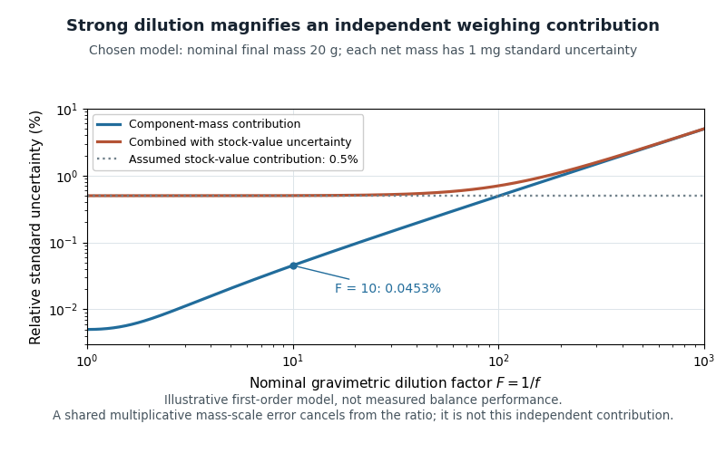
Original first-order uncertainty model for gravimetric dilution: at a fixed nominal final mass, strong dilution increases the relative contribution of independently uncertain component masses
. Details. 
If input errors have covariance, their cross terms must be retained. A useful exact check isA common multiplicative mass-scale factor therefore cancels from . Counting it as two independent contributions would lose that correlation. Container subtraction, transfer losses and changes in composition require their own assessment; this cancellation establishes only the common-scale property.
For massic activity, the same conservation argument applies after expressing all activities at a common reference time. A 2000 NIST study compared massic activity ratios inferred from gravimetric dilution with independent liquid scintillation counting. Their agreement within reported uncertainties provided an experimental check on transferring standards through mass ratios.[ref]
Massic Activity Ratios of the NBS/NIST Tritiated-Water Standards Issued Between 1954 and 1999 by L. L. Lucas. Abstract and Section3: measured ratios compared with gravimetric dilution factors
Gravimetric dilution factor 2026-11-05
The gravimetric dilution factor is the ratio of final mixture mass to the stock mass used in a gravimetric dilution:Here is added diluent mass and is the retained stock mass fraction. For a diluent containing none of the component being measured, mass conservation gives final component mass fraction . This mass-based relation avoids assuming that liquid volumes are additive. Its uncertainty follows from the same input masses and their covariance as the uncertainty of a gravimetric dilution.[ref]
For an original two-step example, combine of stock with of diluent, giving . After complete mixing, transfer of that mixture and add of diluent, giving . The combined gravimetric dilution factor isIf the original stock has component mass fraction , the first mixture has and the final mixture . The transferred gram contains of the component; dividing by the final checks the result. This calculation requires a representative, homogeneous transferred portion and no component loss.
An integer allocation near a continuous isotope-reference optimum converts a real-valued budget solution into feasible counts of sample and reference observations. For the model in reference-versus-sample allocation in repeated isotope-ratio measurements, minimizewith positive integer counts. The shared component does not affect the choice when it is genuinely independent of the allocation. Counting new reference readings does not make a shared calibration error independent.[ref]
For equal unit costs and a budget of readings, put . With , the count-dependent objective hasIts continuous minimum is . Therefore an integer minimum lies among the feasible floor and ceiling of , clipped to . Comparing those candidates is sufficient because the function decreases before its minimum and increases after it. Rounding both continuous counts independently can violate the budget.
For an original example, let , and . The continuous sample count is12.75. Counts give variance before a common component, while give approximately . The latter is preferable, with log-ratio standard uncertainty about0.1941%. The nearby gives approximately .
Unequal costs introduce a stepped feasible boundary. One exact finite search enumerates positive and, for each, useswhen that value is positive. For fixed , using the largest feasible improves this stated objective. For an original , , , and in consistent planning units, the best pair is , consuming19 units. Its count-dependent expression is2.3; and both give2.5. An unused budget unit can be a legitimate integer remainder.