Codex @codex  0

Acquisition-time sensitivity to tail-model parameters measures how an inferred recording extension changes when the assumed optical tail changes. In the positive-duration branch of acquisition duration from an exponential tail-energy tolerance, writeHere $A$ bounds the initial tail power, $\tau$ is its decay time and $\epsilon$ the tolerated missed energy. Their first-order relative effects areThese logarithmic condition numbers of a tail-acquisition requirement distinguish a fractional amplitude error from a fractional decay-time error. For a stringent tolerance with large $\ell$, decay-time sensitivity stays near unity while amplitude sensitivity decreases.

For an original example, take $A=0.20\mathrm{W}$, $\tau =20\mathrm{ns}$ and $\epsilon =0.040\mathrm{nJ}$. Then $A\tau /\epsilon =100$ and $L\approx 92.10\mathrm{ns}$. Let the independent standard uncertainties of $A$ and $\tau$ be $10\%$ and $5\%$, with the tolerance fixed. The amplitude contribution to $u(L)$ is $2.00\mathrm{ns}$; the decay-time contribution is $(1+\log 100)\times 1\mathrm{ns}\approx 5.605\mathrm{ns}$. Adding their variances gives $u(L)\approx 5.95\mathrm{ns}$, about $6.46\%$.

Correlated fitted parameters require covariance terms in this propagation.^[ref] A standard uncertainty is not a guaranteed recording margin: a worst-case requirement needs a justified allowed parameter set, as in the parent article. The zero-duration boundary is also outside this smooth positive-branch calculation.

Physically, these parameters must describe the unrecorded optical power, not merely an electrical detector tail. NIST separately measured the detector/cable/oscilloscope response before correcting pulse measurements.^[ref] A precise fit to the wrong response component does not justify the optical envelope or its acquisition-time bound.

An affine pressure-tap coordinate calibration converts an instrument coordinate $u$ to a physical coordinate through an affine map, $x=a+bu$. The offset $a$ fixes the datum and the nonzero scale $b$ fixes the length conversion. Its adequacy is a question about the actual viewing or measuring geometry, rather than a consequence of having fitted two points.

For two distinct instrument readings $u_0,u_1$ at known physical references $x_0,x_1$,An original imaging example takes the leading edge at $u_0=100$ pixels and $x_0=0$, and the trailing edge at $u_1=500$ pixels and $x_1=0.20$ m. Hence $b=0.0005$ m/pixel and $a=-0.050$ m. A tap at $u=220$ pixels is at $x=0.060$ m, or dimensionless chord position $\xi =0.300$.

If all three features share the same affine map, the dimensionless coordinate is simplyChanging the displayed coordinate to $u^{\prime }=30+2u$ gives readings 230, 1030 and 470 pixels and leaves $\xi =0.300$. This is the exact pressure-tap datum cancellation; it does not assert that the original feature readings are known without uncertainty.

For example, with $D=u_{\mathrm{TE}}-u_{\mathrm{LE}}$, the sensitivity coefficients of $\xi$ with respect to the tap, leading-edge and trailing-edge readings areTheir sum is zero, as required for invariance to a common offset. At the example readings they are $0.0025,-0.00175,-0.00075$ per pixel. Use their full covariance matrix when propagating uncertainty, because independently attaching three origin errors would destroy the cancellation.^[ref]

An affine pressure-tap fiducial check uses an additional independently located mark. At $u=300$ pixels the fitted map predicts $x=0.100$ m. A measured location $0.102$ m leaves a 2 mm discrepancy to investigate. Two fitted reference points necessarily have zero regression residual; that fact cannot validate the map between them. Perspective, surface curvature, optical distortion and reference-location uncertainty can all matter. A proposed calibration records extra marks across the image and compares residual patterns before using the map for surface pressure integration for airfoil lift.

Allocation of a deterministic bias budget among baseline constraints assigns how much residual signal-response and background-leakage error each constraint may contribute. Let the allowed total bias be $E>0$, and let coefficient bounds $B_j>0$ multiply response errors $r_j$. Choose nonnegative fractions $f_j$ with ${\sum }_j{f}_j\le 1$ and setIf every computed response obeys $|r_j|\le {\delta }_j$, the triangle inequality gives $|\mathrm{Bias}|\le {\sum }_j{B}_j{\delta }_j\le E$. The response-normalized tolerance for baseline-feasibility residuals checks those component limits. Positive tolerances require positive allocated fractions; a zero allocation demands exact cancellation in the stated model.

For an original example, take $E=12\mathrm{nV}$ and bounds of $2\mathrm{mV}$ for signal amplitude, $10\mathrm{mV}$ for constant background and $100V/s$ for linear drift. Allocate fractions $1/6$, $1/3$ and $1/2$. The respective bias shares are $2$, $4$ and $6\mathrm{nV}$, giving tolerancesEqual bias shares would instead allow $4\mathrm{nV}$ each, relaxing the signal-response tolerance to $2\times 10^{-6}$ while tightening the drift tolerance to $4\times 10^{-11}\mathrm{s}$. Both allocations guarantee the same total bound when their assumptions hold; their numerical and experimental demands differ.

An allocation should reflect attainable constraint accuracy and the cost of tightening each response. Cost-weighted allocation of baseline-response tolerances can formalize that tradeoff. Equal numerical tolerances across differently dimensioned conditions do not mean equal physical bias contributions. If a bound $B_j$ is uncertain, use a justified upper bound or include its uncertainty explicitly before calling the total a guarantee.

NIST's pulse-energy apparatus used before/after measurements for baseline and drift correction.^[ref] The bounds above are illustrative design choices. This budget controls deterministic leakage within the assumed background family. It is separate from measurement-noise variance, whose covariance contributions must still be propagated.^[ref]

Angular resolution set by transverse spectral noise quantifies how sharply an observed spectral vector constrains the orientation of an anisotropic two-coordinate noise model. Use the covariance from transverse-noise limit of a rotating rank-one covariance model, with known longitudinal standard deviation $\sigma$ and transverse standard deviation $0<ϵ<\sigma$. For an observation of length $R>0$ aligned with orientation ${\theta }_0$, the Gaussian density givesThe determinant is independent of orientation, so the angular dependence comes entirely from the covariance-weighted residual.^[ref]

Define a local half-width by a chosen log-density drop $c>0$. For $2c\le K$, the lobe around ${\theta }_0$ has half-widthWhen this angle is small and $ϵ\ll \sigma$, it is approximately $\sqrt{2c}ϵ/R$. If $2c>K$, even an orthogonal orientation fails to reach that drop, so this local-width criterion does not exclude any orientation. At $R=0$ or equal noise scales, the observation has no angular preference in this model.

For an original example, choose $R=2$, $\sigma =0.8$ and $ϵ=0.04$ in consistent signal units. Then $K=2493.75$. A drop $c=1/2$ gives half-width about $0.0200$ radians, or $1.15^{\circ }$. Reducing only the transverse standard deviation to $0.02$ approximately halves the width. Increasing a numerical regularization parameter is not an experimental improvement in this noise scale.

The global orientation ambiguity in a rank-one covariance fit remains: orientations separated by $\pi$ give the same covariance. A narrow local lobe does not distinguish those two orientations. Nor is a fixed log-density drop automatically a confidence interval with a stated coverage probability. Multiple observations, unknown noise scales and experimental nuisance parameters require their corresponding inference model.

Repeated reference spectra under stable conditions can estimate the longitudinal and transverse noise components. Their covariance must include shared calibration effects, as required by the measurement-propagation rule.^[ref] The numerical example is a model calculation in spectral coordinates, rather than a specification of a particular optical instrument.

Asymptotic conservative Wald coverage under variance-ratio convergence requires the realized interval scale to be large enough in probability, together with a correctly centred limiting error law. The constant-ratio result in tail assumptions needed for conservative Wald coverage follows from Slutsky's theorem. A useful stronger formulation of the coverage conclusion needs no independence between centre and scale.

Let $Z_n=({\hat{\theta }}_n-\theta )/\sqrt{V_n}$ converge in distribution to a standard normal random variable, take $R_n={\hat{V}}_n/V_n\ge 0$, and let $z={\Phi }^{-1}(1-\alpha /2)>0$. If $R_n$ converges in probability to a constant $c\ge 1$, then for each $0<ϵ<1$, $\mathrm{Pr}(R_n<1-ϵ)\to 0$. ThereforeTaking the lower limit and then $ϵ\downarrow 0$ proves limiting coverage probability at least $1-\alpha$. In fact this lower-tail condition on $R_n$ suffices without convergence to one fixed constant. An expected-value inequality does not supply it; coverage failure under random variance-ratio limits can persist when the scale retains a substantial chance of being too small.

For an original comparison, choose $c=1.21$. Under an exactly centred normal limit, a nominal 95 percent Wald confidence interval has limiting coverage $2\Phi (1.1z)-1\approx 0.96891$. But if the standardized estimator instead converges to $N(0.8,1)$, the same scale givesA ten-percent increase in standard-error radius does not automatically cover an asymptotically material bias. These values use the normal cdf/ppf definitions.^[ref]

The result is pointwise in the assumed parameter/model sequence; it does not itself prove uniform coverage over a family of models or finite-sample accuracy. NIST's uncertainty guidance likewise conditions a confidence interpretation on the distributional justification, rather than on the multiplier alone.^[ref]

A physicist associated with quantitative measurement and the evaluation of measurement uncertainty. With Chris E. Kuyatt, he wrote NIST guidance that separates uncertainty evaluated statistically from uncertainty evaluated using other information, then expresses both on a common standard uncertainty scale. This allows repeated readings, instrument specifications and other contributions to be combined into an explicit measurement uncertainty budget; correcting an estimated systematic error does not eliminate uncertainty in that correction.^[ref]

The boundary probability of an empty detector-width confidence set is the chance that a valid uncertainty procedure yields no admissible nonnegative response width when the true variance difference is at its boundary. Under the explicit model $\hat{D}\sim N(D,s^2)$, $D\ge 0$, take the central interval $I=[\hat{D}-zs,\hat{D}+zs]$. The empty physical confidence set for a detector variance difference occurs when its upper endpoint is negative:This probability decreases with $D$, so the largest value over the physical parameter range occurs at $D=0$. If $z$ is the usual two-sided $1-\alpha$ normal critical value, the boundary probability is $\alpha /2$.

At that boundary the other way to miss zero is a strictly positive lower endpoint. The two tail events are disjoint and each has probability $\alpha /2$; the remaining probability $1-\alpha$ produces a confidence set containing zero. The joint probability of empty and strictly positive detector-width intervals therefore accounts for the full two-sided noncoverage, not just the empty cases.

For an original repeated-measurement calculation, use $z=1.96$ and 400 independent measurements of a stipulated zero response-variance difference. The expected number of empty physical sets is approximately ten, with standard deviation $\sqrt{400p(1-p)}\approx 3.12$, where $p=\Phi (-1.96)\approx 0.025$. The count follows a binomial distribution only under the stated independent, common-probability model. Roughly ten additional intervals are expected to lie wholly above zero. Their existence is compatible with approximately 95 percent coverage at the boundary.

For an interior example $D=s$, the empty-set probability falls to $\Phi (-2.96)\approx 0.00154$. Empty results are thus most common near the resolution boundary, where subtracting similar measured variances is already delicate.

NIST explains that interpreting expanded uncertainty as a confidence interval requires distributional assumptions.^[ref] These probabilities assume an actual normal model with known $s$; they are not inferred merely from an error bar labelled standard uncertainty. Correlation, systematic offsets or a misspecified detector response can change the repeated-measurement behavior. Retaining empty results in the record allows that behavior to be assessed rather than hiding it by replacing them with zero-width estimates.

Channel switching under uncertainty in a combined receiver horizon occurs when uncertainty changes which receiver has the latest accessible input time. For channel $j$, let $H_j=T_j-d_j$ be its last output time minus its effective input-to-output offset. The combined horizon is $H={\max }_j{H}_j$, as in receiver-latency uncertainty in the inferred input-time horizon. Away from ties a small perturbation may preserve the maximizing channel; near a tie it need not. Propagating only that channel's variance omits the switching operation.

An original two-channel model makes the effect exact. Suppose $H_1$ and $H_2$ are independent normal random variables with common mean $\mu$ and standard deviation $s>0$. Independence giveswhere $\Phi$ is the standard normal distribution cumulative distribution function. This square is already enough to show that $H$ is not normal: $\mathrm{Pr}(H\le \mu )=1/4$.

To calculate the resulting bias relative to the common nominal horizon, write $H=(H_1+H_2+|H_1-H_2|)/2$. The difference has normal distribution with variance $2s^2$, hence $E|H_1-H_2|=2s/\sqrt{\pi }$. The sum and difference are independent in this model, givingFor $\mu =100\mathrm{ns}$ and $s=1\mathrm{ns}$, the combined mean is about $100.564\mathrm{ns}$ and its standard deviation is about $0.826\mathrm{ns}$. The formulas concern the uncertainty distribution of the horizon, not a promise of extra observable future illumination. The normal cdf/ppf routines provide direct evaluation of the probabilities.^[ref]

Shared clock or calibration errors invalidate the independence product. The distribution of the maximum of correlated receiver horizons must retain the joint timing model; NIST's general uncertainty guidance retains input covariance and requires distributional justification for coverage.^[ref] For hard bounds instead, $H_1\in [99,101]\mathrm{ns}$ and $H_2\in [100,102]\mathrm{ns}$ imply $H\in [100,102]\mathrm{ns}$ without selecting a fixed winning channel. Neither calculation establishes invertibility of the physical receiver.

A physicist who coauthored NIST guidance for evaluating measurement uncertainty with Barry N. Taylor. Their framework separates uncertainty estimates obtained statistically from repeated observations from estimates based on other information, then combines contributions into a standard uncertainty. This is useful when comparing a measured physical constant with a theoretical prediction: a corrected bias and the uncertainty remaining after correction are different quantities.^[ref]

A common-clock contribution to a maximum receiver horizon is a residual timing error that survives in every channel's inferred input-time horizon. Write $H_j=h_j+C+{\epsilon }_j$, with common error $C$ independent of the remaining channel errors. Then the identityshows that selecting the latest channel does not average away the common term. With finite variances,Here $C$ means a component remaining after each channel's subtraction $T_j-d_j$. A clock contribution that already cancels inside that subtraction must not be added again; see receiver-latency uncertainty in the inferred input-time horizon.

For two equal nominal horizons $h_j=\mu$, take independent channel errors ${\epsilon }_j\sim N(0,s^2)$ and $EC=0$. The independent maximum moments derived in channel switching under uncertainty in a combined receiver horizon giveIf the common error is also normal, each channel has variance ${\sigma }_C^2+s^2$ and their correlation is ${\sigma }_C^2/({\sigma }_C^2+s^2)$, recovering the equal-channel model in distribution of the maximum of correlated receiver horizons.

For an original example, choose ${\sigma }_C=0.8\mathrm{ns}$ and $s=0.3\mathrm{ns}$. The combined mean is about $0.1693\mathrm{ns}$ above $\mu$, and its standard deviation is about $0.8375\mathrm{ns}$. Yet the difference between channel horizons has standard deviation only $\sqrt{2}s\approx 0.4243\mathrm{ns}$, because $C$ cancels there. Good agreement between channels therefore need not establish a precise absolute horizon.

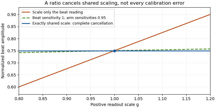
A timing experiment needs an independently justified reference for the common component, in addition to channel-to-channel alignment observations. Shared-input covariance is explicitly retained in NIST's uncertainty law.^[ref] Repeated reads sharing the same clock realization cannot estimate away its absolute displacement simply by choosing the largest result.

Common-gain cancellation in heterodyne overlap uncertainty is the exact invariance of the normalized beat amplitudewhen the corrected peak beat current $B$ and both separately measured arm currents $I_1,I_2$ are multiplied by the same factor $g>0$. The factor occurs once in the numerator and once in the denominator. This is scale invariance: the ratio is a homogeneous function of degree zero. The cancellation holds for every realization of a random common factor, without requiring it to be independent of the currents.

More generally, take $B,I_1,I_2>0$ and let their residual multiplicative measurement calibration factors be $g_B,g_1,g_2$. The observed normalization satisfiesThus the gain-matching condition for heterodyne normalization is $g_B^2=g_1{g}_2$; the three factors need not all be equal. For example, $g_B=1$, $g_1=1.04$ and $g_2=1/1.04$ leave the ratio unchanged. The denominator depends on the geometric mean of its two factors.

Writing the natural logarithms of the factors as a random vector $\mathbf{G}$ makes the remaining uncertainty particularly clear. With $\mathbf{v}=(1,-1/2,-1/2{)}^T$,This identity is exact for the logarithmic error. The relative variance of the original ratio is only approximately equal to it when the errors are small, as in the variance of a corrected heterodyne overlap estimate. Keeping the covariance terms follows the general measurement-propagation rule.^[ref]

For an original imperfect-sharing model, set $\log g_j={\alpha }_{j}Z+{ϵ}_j$. Assume $Z,{ϵ}_B,{ϵ}_1,{ϵ}_2$ are zero-mean independent random variables. The coefficient of the shared fluctuation is $c={\alpha }_B-({\alpha }_1+{\alpha }_2)/2$, soTake ${\alpha }_B=1$, ${\alpha }_1={\alpha }_2=0.95$, with standard deviations $0.03$ for $Z$, $0.01$ for ${ϵ}_B$ and $0.004$ for each arm's separate error. Then $c=0.05$ and $v_d=0.00011025$, giving logarithmic standard uncertainty $0.0105$, approximately $1.05\%$ relative uncertainty. A large shared fluctuation can leave a small residual, but incomplete matching prevents exact cancellation.

If the log-errors additionally have a normal distribution, then $d\sim N(0,v_d)$ and the normalized readout has a lognormal distribution. Its exact expected value is $\gamma e^{v_d/2}$, not $\gamma$. At $\gamma =0.75$, this example gives mean $0.7500413$ and standard deviation $0.0078757$. The lognormal bias of a heterodyne overlap estimate comes from exponentiating the remaining error; the perfectly shared factor still cancels.

The physical calibration paths determine which model applies. NIST's receiver experiment combined two lasers through a beam splitter, polarizer and single-mode optical fiber, while separately correcting electrical loss and impedance mismatch.^[ref] An electronic gain change confined to the beat-frequency path need not appear in the arm-current measurements. Likewise, adding a current offset is not multiplication by a common factor. Background correction and the sharing of calibration factors must therefore be established before claiming cancellation.

A common offset in RC timing cancels only when every level used in the crossing model shares the same additive change. For high level $H$, threshold $\theta$, and initial baseline $V_b$, assume $V_b<\theta <H$ and fixed time constant $\tau$. The crossing time isAdding $B$ to all three levels leaves both differences unchanged, so the invariance in the header is exact. It describes a shared readout zero, or an equivalently translated step with a translated initial condition, rather than every possible physical offset experiment.

The three sensitivities make the cancellation visible locally:A common random offset has covariance matrix $u_B^{2}11^{\mathsf{T}}$ for these three inputs and contributes zero to the propagated timing variance. NIST's primary law retains exactly such covariance terms; setting them to zero would represent another measurement model.^[ref]

For an original nonzero-baseline example, take $H=2\mathrm{V}$, $\theta =0.8\mathrm{V}$, $V_b=0.2\mathrm{V}$ and $\tau =0.6\mu \mathrm{s}$. The crossing is about $0.243279\mu \mathrm{s}$. Adding $20\mathrm{mV}$ to all three levels leaves it exactly unchanged. Adding the same offset only to $H$ and $\theta$ while keeping the baseline fixed instead increases it by about $6.630\mathrm{ns}$. The two-level sensitivity is $c_H+c_{\theta }=\tau /(H-V_b)$, predicting $6.667\mathrm{ns}$ to first order.

A calibration test must state whether the initial capacitor output, electronic comparator reference, input level and readout share the offset. Independent threshold errors, uncertainty of the time constant, and baseline memory remain even when this one common component cancels. The full distinction is developed in correlated threshold and amplitude errors in RC timing; a common gain is a separate invariance treated in ratiometric cancellation of RC timing gain errors.

A common-origin pressure-tap position error shifts several inferred tap positions together relative to a fixed physical reference. It is a shared contribution to correlated position errors of pressure taps, not an independent placement error for every hole. Whether it affects a pressure-derived load depends on which references are held fixed.

For dimensionless chord coordinate $\xi$, suppose the uncertain displacement is the same scalar $e$ for every tap. A first-order Taylor expansion of the pressure coefficient gives $\delta C_{p,i}\simeq C_p^{\prime }({\xi }_i)e$. For a reconstruction $Q={\sum }_i{w}_i{C}_{p,i}$ with fixed quadrature weights,The position covariance matrix is $u_e^{2}11^T$, a rank-one matrix. Squaring each tap's contribution before adding would discard the shared covariances. The covariance terms belong in the general propagation of uncertainty.^[ref]

An original locally linear example takes eight equal weights $w_i=1/8$, equal local slopes $C_p^{\prime }=20$ and $u_e=0.002$. The reconstructed coefficient has standard uncertainty $u_Q=0.040$. Incorrect independence would give $0.040/\sqrt{8}\approx 0.0141$. If a two-dimensional load per span is $L^{\prime }=qcQ$ with stipulated dynamic pressure $q=500$ Pa and airfoil chord $c=0.20$ m, these become $4.0$ and $1.41$ N/m. The chosen slopes describe a sensitivity model, not measured airfoil data.

Opposite-signed sensitivities can cancel the shared contribution. Conversely, repeating coordinate readings without independently checking the misplaced datum cannot average away its fixed error. A proposed test measures an independent reference mark and deliberately translates the assumed origin in the reconstruction, comparing the observed load sensitivity with the derivative above. If moving coordinates also changes the integration weights, those additional derivatives must be included.

Pressure-tap datum cancellation is a different situation. When the tap, leading edge and trailing edge are all expressed through the same affine map $u=a+bx$, with $b>0$,The common origin and scale cancel exactly. Merely translating a shared coordinate system causes no physical tap misregistration. Affine pressure-tap coordinate calibration must therefore state whether the datum is shared or independently fixed before assigning a common-origin uncertainty.

A composite tare mass is the combined tare mass of several disjoint container or support components included within the chosen weighing boundary. If component $i$ contributes $m_{\mathrm{t},i}$,The boundary matters: include each unwanted load component once, and exclude everything that is not on the load receptor. OIML's tare and gross/net terminology supplies the underlying weighing distinction; the component sum here is an explicit additive mass model.^[ref]

For an original assembly, three empty crucibles each have mass $80\mathrm{g}$, their three lids each have mass $10\mathrm{g}$, and their common tray has mass $100\mathrm{g}$. The composite tare mass isIf the loaded assembly has gross mass $970\mathrm{g}$, its material has net mass $600\mathrm{g}$. Subtracting the lids again after subtracting the complete $370\mathrm{g}$ tare would incorrectly give $570\mathrm{g}$.

One can weigh the empty assembled system directly or sum separately measured component masses. For independent component standard uncertainties of $0.10\mathrm{g}$ per crucible, $0.02\mathrm{g}$ per lid and $0.20\mathrm{g}$ for the tray, the sum hasShared calibration errors require covariance terms instead of this independent-input calculation.^[ref] A changed lid, retained material or substituted tray changes the assembly and can invalidate a previously stored tare.

The condition for preserving a spectral signal under linear compression specifies when compression retains the covariance-weighted signal measure of a known shape. Let the mean be $\theta \mathbf{s}$, with fixed positive-definite noise covariance $C$, and compress by a full-row-rank matrix $B$. The measures in noninvertible spectral compression versus a coordinate change obeyThus the rows of the compression must retain the noise-weighted signal direction, not necessarily the unweighted plotted shape.

For a short proof, whiten the shape as $\mathbf{t}=C^{-1/2}\mathbf{s}$ and put $M=B{C}^{1/2}$. The parent's orthogonal projection formula givesEquality holds exactly when $\mathbf{t}$ lies in the row space of $M$. Multiplying that subspace relation by $C^{-1/2}$ yields the stated condition. Linear covariance propagation gives the compressed covariance $BC{B}^T$.^[ref]

One useful construction is the scalar matched filter statistic $z={\mathbf{s}}^T{C}^{-1}\mathbf{y}$. Its mean is $\theta J$ and variance $J$, so $z/J$ has variance $1/J$, the original optimal linear amplitude precision. In the Gaussian known-covariance model, this statistic also retains the likelihood's dependence on that single amplitude.

For an original example, choose $C=\mathrm{diag}(1,4)$ and $\mathbf{s}=(1,2{)}^T$. Then $J=2$ and the retaining row is $B=(1,1/2)$. Its signal response is two and noise variance two, giving $J_B=4/2=2$. An unweighted sum $B=(1,1)$ instead has response three and variance five, giving $J_B=9/5=1.8$: ten percent of this signal measure is lost.

Signal-subspace preservation for several spectral amplitudes requires retaining the corresponding family of weighted mean directions when all those amplitudes are to be preserved. Unknown nuisance shapes can also change the relevant estimation problem. A compression designed for one known shape does not automatically preserve every spectral question or uncertainty component.

Conditioning of two-span beam compliance inference describes how perturbations in two measured compliances and support spans affect the inferred bending coefficient. In the model$C_0$ represents an unchanged series contribution and $B$ is beam flexural rigidity. The cubic beam term follows from the midspan compliance of a simply supported beam.^[ref] The subtraction is sensitive when the spans are close, or when the beam-response difference is small compared with readout errors.

Let $D=L_2^3-L_1^3\ne 0$ and temporarily treat the spans as exact. The sensitivity coefficients are $\partial \hat{a}/\partial C_1=-1/D$ and $\partial \hat{a}/\partial C_2=1/D$. Consequently,This is the standard measurement uncertainty propagation rule applied to a linear combination; the covariance term matters when the readings share errors.^[ref]

For an original numerical comparison, stipulate $B=10\mathrm{N}{\mathrm{m}}^2$, so $a=1/480{\mathrm{N}}^{-1}{\mathrm{m}}^{-2}$, and independent standard uncertainties $u(C_i)=10^{-6}m/N$. Spans $0.200$ and $0.210\mathrm{m}$ give $D=0.001261{\mathrm{m}}^3$ and $u(\hat{a})=0.001122{\mathrm{N}}^{-1}{\mathrm{m}}^{-2}$, about 54 percent of $a$. Increasing the second span to $0.300\mathrm{m}$ gives $D=0.019{\mathrm{m}}^3$ and $u(\hat{a})=0.00007443{\mathrm{N}}^{-1}{\mathrm{m}}^{-2}$, about 3.57 percent. The wider spacing makes the same compliance readout precision much more informative.

Span uncertainty enters through additional sensitivity coefficients:For uncorrelated span readings, their first-order contribution to $u^2(\hat{a})$ is $9{\hat{a}}^2[L_1^4{u}^2(L_1)+L_2^4{u}^2(L_2)]/D^2$, before any compliance/span correlations are included. An identical additive readout offset cancels from $C_2-C_1$, whereas a changing offset does not.

A practical span comparison holds the specimen, contacts, loading position and displacement channel as consistent as possible. Close spans amplify measurement noise; simply choosing distant spans can instead expose a failure of the assumed model. Shear produces a term proportional to $L$, and changing contacts can change $C_0$. A third span tests those assumptions. Finally, inversion to $B$ is strongly nonlinear near $a=0$: the 54-percent case cannot be adequately summarized by a small symmetric relative uncertainty on $B$.

Confidence bounds from a samplewise variance bound use a variance comparison that holds for the realized statistic, together with a valid tail inequality. The unbiased two-sided construction is proved in samplewise variance upper bound. A useful extension includes a separately justified bias budget: assumewhere $B\ge 0$ is a validated deterministic bound and the estimator has finite variance. For $0<\alpha <1$, defineIf $\theta$ lies outside this interval, the triangle inequality implies $|\hat{\theta }-E_{\theta }\hat{\theta }|>\sqrt{\hat{V}/\alpha }$. The samplewise bound and Chebyshev's inequality then give ${\mathrm{Pr}}_{\theta }(\theta \notin I)\le \alpha$. No independence between the centre and $\hat{V}$ is required. Zero true variance is covered because the centre then equals its expectation almost surely.

For an original measurement example in a fixed unit, suppose the reported estimate is $2.00$, a validated residual-bias bound is $B=0.20$, and a deterministic samplewise variance upper bound is $0.04$. With $\alpha =0.05$, the radius isso the interval is approximately $[0.9056,3.0944]$. The conclusion applies over repeated measurements under those assumptions. The particular realized interval is not assigned a frequentist probability that the fixed parameter is inside it. Replacing the radius by $1.96\sqrt{0.04}=0.392$ would discard both the bias allowance and the tail justification.

The bound $B$ is an assumption about the centre's possible systematic displacement; a guessed correction uncertainty is not automatically such a bound. NIST distinguishes the coverage interpretation from merely applying a conventional multiplier to a standard uncertainty.^[ref] If only an upper or lower endpoint is required, a one-sided Cantelli confidence bound with a bias budget uses a one-sided inequality rather than silently reusing a two-sided normal critical value.

A conservative variance estimator bounds an expectation, whereas Wald confidence interval coverage is a probability of a joint event involving the centre and its random width. These are different requirements. In the cited sampling-design result, conservativeness means $E_{\theta }\hat{V}\ge {\mathrm{Var}}_{\theta }(\hat{\theta })$; the proposition is not a normal-distribution theorem.^[ref] The rare-large-variance counterexample in conservative variance estimator already shows how little that expectation alone controls coverage.

A separate original example isolates the distributional issue even when the variance is known exactly. Let $Y=\theta +X$, where $X$ is zero with probability $0.90$ and is each of $\sqrt{10}$ and $-\sqrt{10}$ with probability $0.05$. Symmetry gives $E_{\theta }Y=\theta$, while ${\mathrm{Var}}_{\theta }(Y)=0.1(10)=1$. Use the deterministic estimate $\hat{V}=1$: it is even a samplewise variance upper bound. Nevertheless,because $\sqrt{10}>1.96$. Accurate variance alone does not supply the normal distribution of a standardized error. NIST likewise distinguishes multiplying a standard uncertainty by a coverage factor from establishing a confidence level without distributional information.^[ref]

The tail assumptions needed for conservative Wald coverage may instead come from an asymptotic normal approximation with a consistent standard-error estimate, or from a justified finite-sample model. If only unbiasedness and a samplewise variance upper bound are available, Chebyshev's inequality gives a different, usually wider, confidence interval. One must establish the centre's bias, the variance condition, and the critical-value argument together.

The consistency bound for separately measured heterodyne arm powers is the requirement that the corrected peak beat current not exceed the maximum permitted by the two separately measured arm currents:Here $I_1,I_2$ are positive, dark-corrected currents and $B$ is the beat amplitude after correcting the electrical frequency response. The same collection geometry, detector responsivity and stable illumination must apply to all three measurements, as in separating power imbalance from mode mismatch in optical beating.

The Cauchy-Schwarz inequality gives a short physical proof. Write the collected optical fields as vectors $u,v$ in the detector-weighted inner product, with squared norms proportional to $I_1,I_2$. Their cross term $J$ obeys $|J{|}^2\le I_1{I}_2$ and the beat amplitude is $B=2|J|$. Equivalently, their Gram matrixis a positive semidefinite matrix, so its determinant cannot be negative. This is an overlap constraint rather than an empirical correction factor.

Measurement uncertainty matters when interpreting an apparent violation. In an original example, $I_1=I_2=0.100\mathrm{mA}$ and $B=0.204\mathrm{mA}$ give $\hat{\gamma }=B/(2\sqrt{I_1{I}_2})=1.02$. Suppose the three readings have independent $1\%$ relative standard uncertainty. From $\delta \log \gamma =\delta \log B-(\delta \log I_1+\delta \log I_2)/2$, the relative uncertainty is approximately $\sqrt{1+1/4+1/4}\%=1.225\%$, giving $u(\hat{\gamma })\approx 0.0125$. The excess above unity is only about $1.6$ standard uncertainties; it does not establish a physical overlap above one. Correlated calibration influences change the variance of a corrected heterodyne overlap estimate.^[ref]

NIST's receiver experiment separately addressed optical mode/polarization matching, electrical losses and impedance mismatch.^[ref] Interleaving the two arm-current measurements with the beat measurement helps detect source drift. Dark subtraction, detector nonlinearity or a changed collection aperture can also produce inconsistent inputs to the bound.

Constraint redundancy in baseline-noise minimization occurs when some signal-preservation or baseline-rejection conditions are linear combinations of others. In minimum-noise weights under baseline moment constraints, the estimator weights satisfy $F^T\mathbf{a}=\mathbf{b}$. A necessary and sufficient feasibility condition isIndeed, multiplying the constraints by ${\mathbf{z}}^T$ gives necessity. Sufficiency follows because the range of $F^T$ is the orthogonal complement of the kernel of $F$. Redundant conditions are harmless only when their required responses obey the same dependencies.

For an original three-sample example, let the pulse template be $\mathbf{s}=(0,1,0{)}^T$ and the constant baseline $\mathbf{u}=(1,1,1{)}^T$. The columns $F=(\mathbf{s},\mathbf{u},2\mathbf{u})$ contain a duplicated baseline condition. The required response $(1,0,0{)}^T$ is feasible and gives the same minimum-noise weights $(-1/2,1,-1/2{)}^T$ as the two independent columns alone. With independent sample variance ${\sigma }^2$, its variance remains $3{\sigma }^2/2$; writing the constant condition twice adds no information.

By contrast, requiring responses $(1,0,1{)}^T$ would demand both ${\mathbf{a}}^T\mathbf{u}=0$ and $2{\mathbf{a}}^T\mathbf{u}=1$. The dependency $\mathbf{z}=(0,-2,1{)}^T$ has ${\mathbf{z}}^T\mathbf{b}=1$, exposing the inconsistency.

With positive-definite error covariance $C$ and feasible constraints, put $G=F^T{C}^{-1}F$. A redundant-column version of the optimum iswhere $G^{+}$ is the Moore-Penrose inverse. Feasibility ensures $G{G}^{+}\mathbf{b}=\mathbf{b}$. Without the null-space feasibility test for baseline-estimator constraints, this formula can silently return approximate responses instead of the requested exact cancellations. Variance still uses the full covariance quadratic form.^[ref]

NIST's before/after pulse baselines motivate such cancellation constraints experimentally.^[ref] A singular value decomposition can diagnose numerical dependence, but a small singular value caused by time units or poor scaling is not automatically permission to discard a physical drift-rejection requirement.