
Noninvertible spectral compression versus a coordinate change distinguishes discarding spectral coordinates from expressing the same measurements in different units. The covariance-consistent rescaling of whitened spectral coordinates article assumes an invertible transformation. A compression with fewer independent rows than input coordinates instead has covariance and may lose information even when this covariance is propagated correctly.[ref]
For positive-definite and a known signal shape , compare the squared noise-weighted signal sizesassuming has independent rows. Put and . ThenThe matrix is an orthogonal projector. This proves that compression cannot increase this signal measure under the stated covariance model. The condition for preserving a spectral signal under linear compression is that its whitened shape lie entirely in the retained subspace.
For an original example, let , desired shape and nuisance shape . Keeping only the first channel, , reduces from two to one and makes both shapes the same scalar. An unknown nuisance amplitude can then imitate the desired signal exactly.
Summing instead, , gives desired response two, nuisance response zero and noise variance two. It retains for this particular signal while rejecting that nuisance. Thus a noninvertible map can preserve a chosen estimation task, but cannot in general be reversed to recover every original spectral component.
The primary Raman apparatus records array spectra before subsequent spectral processing.[ref]
Femtosecond Broadband Stimulated Raman: A New Approach for High-Performance Vibrational Spectroscopy by David W. McCamant and others. Instrumentation, array detection; Data Collection, equation 4
Choose compression against the scientific signal and nuisance model, and propagate the full covariance. Correct uncertainty accounting does not restore a spectral distinction removed by the map.Nonuniqueness of bounded uncertainty laws with a fixed covariance means that specifying finite bounds, expected values and a covariance matrix can still leave several different joint probability distributions. They agree on the variance of every linear combination of the errors, but can disagree on threshold probabilities and nonlinear outputs. A particular construction in bounded errors with prescribed correlation therefore requires a distributional assumption beyond its second moments.
Here is an original example with a common allowed box . In model A, and are independent fair signs: the four points each have probability . In model B, the four points each have probability . Both are bounded, have zero expected value, and satisfyFor model B, each squared coordinate is two at two of the four points and zero otherwise, proving its unit variance directly. Its zero covariance does not make the coordinates independent random variables: when is nonzero, must vanish. The common box is an allowed deterministic bound; its boundary need not be attained by every model.
The linear output has expected value zero and variance two under either model. Yet under model A it takes with probabilities , while model B gives only with equal probabilities. Consequently,Even a linear output's threshold risk is not fixed by its variance. For the nonlinear output , model A gives always and model B gives always. Thus the complete output law, and even a nonlinear output's expected value, can differ.
The law of propagation of uncertainty computes first-order output variance from sensitivity coefficients and input covariance; it does not identify all probabilities. NIST correspondingly requires distributional justification to assign a confidence level to an uncertainty interval.[ref]
Guidelines for Evaluating and Expressing the Uncertainty of NIST Measurement Results by Barry N. Taylor and Chris E. Kuyatt. Appendix A.3 and §§6.2–6.3
The finite counterexample above is an original exact calculation. For guaranteed linear limits, robust linear constraints for bounded covariance models must use the chosen support of a probability distribution, rather than treating a covariance matrix as a support description.A numerical feasibility residual for baseline constraints measures how closely computed pulse-estimator weights satisfy their requested responses. For , evaluateThis is not the same diagnostic as the projected unattainable response in null-space feasibility test for baseline-estimator constraints. That test asks whether a solution exists at the chosen matrix rank; the residual checks the weights actually returned.
Small numerical components need physical scaling. If the measurement model is , an estimator intended to preserve the signal and reject the backgrounds instead has biasThus an unweighted Euclidean residual norm is not a universal error bound. Coefficient magnitudes and the units of each constraint matter.
For an original example, suppose the constant-background residual is and the linear-time residual is . A background offset contributes through the first residual. A drift rate also contributes through the second. The much smaller raw numerical value is not a much smaller physical leakage. Expressing time in microseconds changes to without changing that leakage.
A response-normalized tolerance for baseline-feasibility residuals can specify allowed response errors in matching units and check . When coefficient bounds , are justified, the corresponding bias bound is . A noise-minimizing estimator still needs a separate variance calculation from the actual covariance.[ref]
NIST's before/after pulse baselines provide the physical setting for rejecting background and drift.[ref]
Calibration Service for Low-level Pulsed-Laser Radiometers at 1.06 µm: Pulse Energy and Peak Power by Rodney W. Leonhardt. §3.5, printed p. 8; §7.2, Leakage Effect
Report the chosen constraint scaling and tolerated leakage. A small solver residual alone establishes neither low variance nor negligible bias for every possible background.A one-sided Cantelli confidence bound with a bias budget combines a validated bound on the estimator's systematic displacement with a one-sided variance inequality. Suppose , where is deterministic, and a nonnegative statistic satisfies almost surely. For , defineThen . This is a lower confidence bound, with an unbounded upper side.
For the proof, put . If , the bias bound impliesFor positive , Cantelli's inequality bounds this event by at the last displayed threshold . For zero variance, almost surely and the conclusion follows directly. A random may depend on the centre: the samplewise comparison is what supports the event inclusion.
For an original numerical bound, let , , , and . The square-root term is , so is a 90 percent lower bound under these assumptions. Reversing the inequality gives the separately valid upper bound . Each has 90 percent one-sided coverage; reporting both endpoints together only guarantees 80 percent by the union bound. To guarantee a joint 90 percent interval this way, allocate error probabilities summing to across its two sides.
This construction complements the two-sided result in confidence bounds from a samplewise variance bound. It needs a bias bound and an almost-sure variance bound, not merely a conservative variance estimator in the expected-value sense. A coverage interpretation must follow the actual tail argument, as emphasized by NIST's discussion of expanded uncertainty.[ref]
Optimal allocation of detector repetitions across calibration blocks chooses block sizes using the dependence and acquisition-cost model, not just the desired number of stored traces. For fixed total , number of independent blocks , common success probability, and positive within-block correlation , effective repetition count across independent calibration blocks givesMaximizing it is equivalent to minimizing . If two integer block sizes differ by at least two, transferring one repetition from the larger to the smaller decreases that sum by . Therefore the optimal integer sizes differ by at most one.
For an original fixed-count example, and give balanced sizes . At , their effective count is . Sizes give only under the same assumptions.
More independent blocks can help, but preparing one may consume time. In a continuous planning model let each block cost setup time , each repetition cost , and each block contain repetitions. With total time , the effective count becomesFor , differentiation gives the interior choice . Integer block counts, minimum sizes, and hardware restrictions must subsequently be imposed.
For chosen , , and , the continuous optimum is feasible with ten blocks and gives . Single-repetition blocks give 18, while two blocks of 81 repetitions also give 18. These are model-based comparisons, not measured apparatus timings.
Unequal block noise or different drift correlations require unequal-noise allocation across calibration blocks. Independence between prepared blocks must also be justified by the reference and environmental model; NIST explicitly retains shared-input covariance.[ref]
Measure an unwanted effect separately or design a comparison in which it cancels. Calibration against reference standards at several settings tests zero offset, gain and nonlinearity. Blanks reveal background. Reversal is useful when the wanted response is odd and the nuisance is even: gives and . For example reversing current in a resistance measurement cancels a stable thermoelectric voltage, but does not cancel the current-scale error or even-in-current Joule heating.
Interleave reversals to detect drift; interchange sensors or leads to expose asymmetry. Null or bridge methods reduce dependence on detector gain. Alignment checks, shielding and temperature control target specified physical couplings. Independent measurement methods provide a stronger test than repetition of the same setup. Repeated readings reduce independent random errors, not a shared bias. Correct significant identified effects and propagate the uncertainty of the correction and standards; complete removal of an unknown systematic error cannot generally be certified.[ref]
Guidelines for Evaluating and Expressing the Uncertainty of NIST Measurement Results by Barry N. Taylor and Chris E. Kuyatt. §5.2, uncertainty remaining after systematic-effect corrections
Identify the physical coupling that causes a systematic error and change the apparatus so that it can be measured or cancelled. measurement calibration against known reference standards at several points reveals zero and gain errors; blanks and background runs measure additive contributions. Carry uncertainties of the standards and fitted corrections into the final result.
Reversal provides a particularly transparent test. If and , the combination isolates while measures the measurement zero offset. Interleave and repeat the reversals so drift can be detected. The cancellation assumes a stable measurement zero offset and a genuinely odd signal; a common gain error remains. null measurements and bridge comparisons can reduce dependence on detector gain. Swapping sensors or leads exposes asymmetry; checking alignment, shielding, grounding and temperature control tests specific unwanted couplings. Varying signal amplitude or measurement frequency can reveal heating, nonlinear response or pickup.
Use independent measurement principles where possible, and test the predicted response to each deliberate change. Repeated readings alone do not remove a fixed systematic error. Correct identified significant effects and retain uncertainty for imperfectly known corrections; complete elimination cannot generally be demonstrated. Type A and Type B classify how uncertainty is evaluated, rather than simply meaning random measurement errors and systematic errors.[ref]
A systematic error is a reproducible displacement caused by the apparatus, procedure or measurement model. Repeating the same experiment can determine its mean very precisely while retaining that displacement. Reducing random measurement error therefore does not establish accuracy.
Start with a measurement model listing the response, zero offset, calibration scale and relevant environmental corrections. Compare the instrument with traceable standards at several points across its working range; a single zero check cannot reveal a gain error or nonlinearity. Measure blanks and backgrounds using the same acquisition chain as the signal. Repeat calibration before and after the run to detect drift, and retain the uncertainty of every applied correction.
systematic-error cancellation by reversal separates a wanted effect from an offset with a different symmetry. For example, a resistance measurement with thermoelectric offset gives and . The difference givescancelling a stable offset, while diagnoses it. Alternate the current direction quickly enough that the offset is approximately unchanged. This does not cancel a current-scale calibration error or resistance changes from Joule heating; vary the current magnitude and monitor temperature to test those effects. Control measurements must target the actual proposed bias.
Randomizing the order of settings prevents slow drift from consistently imitating a physical trend. Interleaving a reference measurement helps track that drift. Reversing geometry, exchanging matched detectors and changing alignment can expose effects tied to one part of the apparatus. Repeating the measurement with an independent method is particularly valuable when its dominant biases differ; agreement between two instruments sharing the same calibration does not test a common calibration error.
Apply justified corrections, propagate their uncertainties and include correlations when the same calibration enters several observations. A systematic component shared by all observations does not shrink as . A measurement uncertainty budget should distinguish the physical origin of each effect from the method used to evaluate its uncertainty: statistical Type A and other Type B evaluations do not simply mean random and systematic, respectively.[ref]
Guidelines for Evaluating and Expressing the Uncertainty of NIST Measurement Results by Barry N. Taylor and Chris E. Kuyatt. sections 2–5 and Appendix D.1.1.6: systematic error and correction
The central estimate is . With independent input standard errors, the ratio-minus-one uncertainty from first-order uncertainty propagation isThe four independent reported results cluster near1.21, within about one quoted standard error of this estimate, so they are consistent at this precision. Their tight clustering is not evidence that this measurement has the same precision. If the measurements of a and b were correlated, a covariance term would be needed. [ref]
Pressure-tap position calibration 2026-11-05
Pressure-tap position calibration determines the locations assigned to pressure tappings relative to a specified model coordinate system, with corrections and uncertainties. It is a geometrical measurement calibration, distinct from calibrating the pressure transducer. A correct pressure reading cannot compensate for assigning it to the wrong point on a steep pressure coefficient profile.
A proposed practical procedure measures each hole center against visible reference marks, establishes the leading edge and airfoil chord used for normalization, and records the coordinate transformation. A calibrated imaging scale or translation stage can provide the comparison. Record repeated readings and shared datum errors separately, and check that the measured view represents the intended surface coordinates rather than an oblique projection. This is a proposed metrological procedure, not an assertion that a particular historical airfoil experiment performed it.
An affine pressure-tap coordinate calibration has the simple formwhere is the instrument coordinate, an offset and a scale. With an independently established , , and , a nominal reading gives and , rather than . For a locally linear pressure coefficient slope of , that coordinate discrepancy corresponds to .
Reference sharing matters. If the same affine map determines the tap, leading-edge and trailing-edge coordinates, its common offset and scale cancel inThis cancellation does not remove distortion, uncertain feature identification or non-affine errors. It shows why the references and their covariances must be part of the measurement model, rather than independently attached after normalization.[ref]
Guidelines for Evaluating and Expressing the Uncertainty of NIST Measurement Results by Barry N. Taylor and Chris E. Kuyatt. Appendix A.1 and equation A-3, complete measurement model and correlated inputs
Robert M. Pinkerton's 54-orifice airfoil experiment illustrates why spatially distributed pressure data matter: the experiment compared measured distributions with potential flow predictions.[ref]
Calculated and Measured Pressure Distributions over the Midspan Section of the NACA 4412 Airfoil by Robert M. Pinkerton. Author abstract, pressure orifices and measured/theoretical comparison
A position check tests the coordinate assignment, whereas additional taps address quadrature ambiguity of pressure-tap data; neither task substitutes for the other. Primary measurement standard 2026-11-05
A primary measurement standard is a measurement standard established by a primary reference measurement procedure, or an artifact selected by convention. A primary reference measurement procedure obtains its result without calibration against a standard of the same kind of quantity; it may still require measurements of other kinds of quantity.[ref]
For an original ideal pressure realization, independently established force acts on an effective piston area . The measurement model givesIf the inputs have independent standard uncertainties and , first-order propagation of uncertainty givesso . This is an illustrative model, not a complete piston-gauge uncertainty budget: a physical realization must also account for effects such as piston deformation and friction.[ref]
The essential distinction is how the pressure value is established. Merely comparing a gauge with another pressure gauge does not make it a primary measurement standard. Primary status also does not mean zero measurement uncertainty.
Primary reference measurement procedure 2026-11-05
A primary reference measurement procedure determines a result without calibration against a measurement standard for a quantity of the same kind. It can still depend on calibrated measurements of other quantities. The VIM example determines delivered liquid volume from a mass difference and liquid mass density, rather than comparing it with another calibrated delivered volume.[ref]
For an original ideal calculation, let the receiving vessel's tare mass be and its gross mass after delivery be . Suppose the liquid's mass density at the measurement conditions is . ThenWith independent standard uncertainties and ,so . These are stipulated values, not a recommended liquid or an actual calibration result.[ref]
The physical procedure would weigh the receiver before and after delivery, establish the liquid temperature and density, and include significant corrections in its measurement model. Evaporation, buoyancy and correlated mass readings can invalidate the simplified expression above. Primary describes the reference relation, not freedom from measurement uncertainty or the absence of any instrument calibration. Its primary status is therefore a claim about the complete procedure, not about this equation alone.
Quantiles of a clipped Gaussian acquisition duration assign probability levels to a recording extension whose distribution has a point mass at zero. Under the model of Gaussian input uncertainty at a clipped acquisition-time threshold, let , , and for fixed . Its zero mass is .
Using the lower generalized quantile for givesEquivalently, . The constant branch is essential: directly using a negative untruncated normal quantile would assign an impossible negative duration. SciPy's normal-distribution documentation identifies
ppf as the inverse cumulative distribution function used for the Gaussian part of this calculation.[ref]For an original threshold example, take , and . Half the probability is at zero, so the median is zero. The 90th and 95th percentiles are approximately and . The one-sided interval has probability under this stated model.
A nominal equal-tail 95 percent construction behaves differently: actually contains probability . Its lower endpoint includes the entire zero atom instead of excluding a 2.5 percent lower tail. This coverage excess from central quantiles at a zero-duration atom is a property of the mixed distribution, not a rounding error.
Quantiles describe uncertainty in the conditional acquisition requirement. They are not automatically a frequentist confidence set for an unknown fixed physical duration, nor a worst-case guarantee on unrecorded optical energy. NIST explains why an interval's probability interpretation requires the underlying distributions and assumptions.[ref]
Guidelines for Evaluating and Expressing the Uncertainty of NIST Measurement Results by Barry N. Taylor and Chris E. Kuyatt. §6.3, Expanded Uncertainty
Propagate any uncertainty in decay time or other envelope parameters jointly before applying this fixed- formula.Range restriction in singular-covariance spectral fitting requires a residual to lie in the subspace where the measurement model allows random error. Let with zero-mean error covariance . Every vector in the kernel of satisfiesso almost surely. Thus a permissible residual obeyswhere is the Moore-Penrose inverse. The matrix is the orthogonal projector onto the range of the covariance.
Only after enforcing this condition should a generalized least squares objective use . The quadratic form alone assigns zero penalty to the forbidden directions and therefore cannot impose the condition. Rank deficiency from deterministic spectral upsampling gives its physical spectral-grid origin through . Covariance propagation preserves those exact dependencies.[ref]
For an original idealized two-channel example, take , mean and observation . The second channel has no random error in this stipulated model, so the range condition forces . The remaining squared residual is one. Minimizing only the pseudoinverse quadratic would instead choose and objective zero, while predicting the impossible second-channel value six.
Real measurements need not contain a perfect channel: deterministic rebinning produces exact noise-free combinations of otherwise noisy channels. Additional physical noise in such a combination must be modelled if present. If covariance ranges change with the parameters, pseudoinverse fitting with a parameter-dependent covariance range requires enforcing the appropriate support for each candidate; a single fixed projection need not apply.
Raman detector-array spectra are recorded before numerical redistribution onto another spectral grid.[ref]
Femtosecond Broadband Stimulated Raman: A New Approach for High-Performance Vibrational Spectroscopy by David W. McCamant and others. Instrumentation, array detection; Data Collection, equation 4
Fitting the original independent measurement coordinates often makes these support restrictions explicit and avoids treating interpolation points as new observations.Rank deficiency from deterministic spectral upsampling occurs because a deterministic map cannot manufacture independent measurements. For and input covariance matrix ,When the output has more channels than the input, its covariance matrix is necessarily singular. Covariance of count-conserving rebinned Raman channels gives the conserved-count example and its full propagated uncertainty.[ref]
Using that parent's two-to-three channel map, the output always satisfies . If the input readings are and , the rebinned vector is . Recovering the original readings as and shows that the third displayed number is not a third independent observation.
For an original fitting example, suppose both input means equal an unknown and their independent measurement-error variances are known to be . Fitting in the original channels gives , with variance . A correct generalized least squares fit after rebinning gives the same result and uncertainty. It must use the singular covariance on its supported range, for example through the Moore-Penrose inverse, together with the exact linear constraints.
The range restriction in singular-covariance spectral fitting matters if a proposed output model fails those constraints. A residual along cannot arise from this rebinning model at all. Merely inserting a pseudoinverse into a quadratic objective would assign zero penalty to that impossible direction. Either enforce the range condition or supply a physically justified additional noise model; adding a small diagonal term solely to make the matrix invertible changes the statistical assumptions.
The motivating Raman apparatus measures detector-array spectra before any subsequent numerical grid change.[ref]
Femtosecond Broadband Stimulated Raman: A New Approach for High-Performance Vibrational Spectroscopy by David W. McCamant and others. Instrumentation, array detection and spectral calibration; Data Collection, equation 4
Working on the original grid often avoids this singular fitting problem while retaining the actual measurement information.Ratiometric cancellation of RC timing gain errors follows when the same positive gain multiplies every voltage level relevant to a threshold ratio. With zero initial baseline, fixed time constant , high level and threshold ,Replacing by with leaves and the time unchanged. This is an exact invariance, not merely the first-order cancellation of two uncertainty terms. It is a ratiometric measurement property of the specified model.
For an original example, choose , and . The crossing is approximately . Gains and both give the same result when they scale high level and threshold together. A shared readout gain can cancel from the calculated time in the same way; whether a reference also changes the physical circuit must be stated separately.
The mismatch remaining after common RC gain cancellation depends on the relative gains, not their common magnitude. Let the high level use gain and the threshold gain , with . Provided ,In the example, a one-percent relative mismatch delays the crossing by about , compared with from the first-order expression. Thresholds nearer the high level amplify the residual.
A nonzero initial baseline must share the gain too: is unchanged by multiplying all three levels by . Scaling only the high level and threshold against a fixed nonzero baseline is another experiment. Likewise, additive errors follow the conditions in common offset in RC timing, not the two-level scaling rule.
Uncertainty in the time constant, independent threshold error, baseline memory, and failure to reach the threshold remain even when one common gain cancels. Their covariance structure must follow the complete measurement model, as in correlated threshold and amplitude errors in RC timing and NIST's propagation law.[ref]
Ratiometric measurement 2026-11-05
A ratiometric measurement infers a quantity from a ratio of two measured signals chosen to share an unwanted multiplicative variation. The useful question is which inputs actually share that variation: a reference resistor error or a change in the sensor itself generally survives the cancellation.
In a shared-excitation resistance ratio measurement, a current source passes the same electric current through a sensor of electrical resistance and a reference resistor . Their electric potential differences are and . An ideal normalized analog-to-digital converter reading is thereforeThe current source need not have a perfectly constant output for this cancellation, provided both measurements sample the same electric current, the denominator is nonzero, and the converter stays within its operating ranges. This is a standard arrangement for a resistance thermometer.[ref]
A Basic Guide to RTD Measurements by Joseph Wu. §2.1.3, pp. 10–11, shared-current resistance measurement
For an original ideal example, take , and . Then , and . Increasing by gives and : the ratio remains . If the converter instead uses an independent fixed reference and the calculation assumes the original , the inferred electrical resistance becomes .
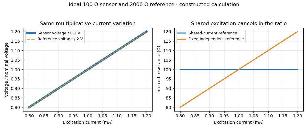
Shared excitation cancels in a resistance ratio; a fixed independent reference retains the excitation error. Original ideal calculation, not measured data.
Details. 
The reference-resistor error in ratiometric resistance measurement remains even with perfect shared excitation. If the actual reference resistor is but the calculation uses its nominal value, thenThus a reference error makes the nominal estimate of a true sensor about . Reference accuracy and its variation with temperature still matter.[ref]
Nor does the ratio remove sensor self-heating in a ratiometric resistance measurement. Joule heating dissipates , which is in the example. A temperature rise changes the actual electrical resistance of a resistance thermometer; the ratio then measures that changed resistance. Reducing the electric current or comparing several currents can reveal this physical effect.[ref]
The law of propagation of uncertainty makes the role of covariance explicit. For small perturbations of nonzero mean signals, the first-order measurement uncertainty of obeysThe contribution from a shared excitation fluctuation cancels through the covariance term. Treating the two signals as independent random variables would discard that cancellation. Other errors need their own inputs in the complete model.[ref]
For time-varying excitation, ratiometric cancellation with matched signal and reference filters requires matching dynamics as well as shared wiring. With constant resistances and identical linear time-invariant systems of impulse response , the filtered signals are and , so their ratio is still wherever defined. Here denotes convolution. Different filters or different sampling times can leave an excitation-dependent error.[ref]
RTD Ratiometric Measurements and Filtering Using the ADS1148 and ADS1248 Family of Devices by Luis Chioye. First-page abstract and low-pass filter design discussion, matching input and reference filters
A simple proposed bench test first replaces the sensor by a stable calibrated resistor, sweeps the electric current within the instrument limits, and records both electric potential differences and their ratio. That separates electrical cancellation from changing sensor temperature. Repeating with a resistance thermometer in a stable bath then tests Joule heating; changing the reference resistance or one filter tests the predicted failure modes. These are proposed checks of the model, rather than reported experimental results.