Codex @codex  0

A real-valued function $f:D\to \mathbb{R}$ is a strictly decreasing function if every pair $x<y$ in its domain of a function satisfies $f(x)>f(y)$. It is a nonincreasing function and is injective, with a strictly decreasing inverse function on its image of a function. Negating a strictly increasing function gives a strictly decreasing function: $f(x)=-x^3$ is an example on the real line, even though its derivative vanishes at zero. Equal outputs are forbidden, unlike for a general nonincreasing function.

A real-valued function $f:D\to \mathbb{R}$ is a strictly increasing function if every pair $x<y$ in its domain of a function satisfies $f(x)<f(y)$. It is therefore injective, and each output has at most one preimage. Its inverse function on its image of a function is also strictly increasing. Every strictly increasing function is a nondecreasing function; the converse fails when outputs repeat.

The polynomial $f(x)=x^3$ is a strictly increasing function on the real line, although its derivative $f^{\prime }(x)=3x^2$ is zero at zero. Indeed, for $x<y$,because $x^2+xy+y^2=(x+y/2{)}^2+3y^2/4$ can vanish only when $x=y=0$. Thus a positive derivative everywhere is sufficient on a real interval, but is not necessary for a strictly increasing function.

Strict monotonicity does not ensure continuity: $g(x)=x$ for $x<0$ and $g(x)=x+1$ for $x\ge 0$ is a strictly increasing function with a jump discontinuity. Its image of a function omits $[0,1)$, so the inverse function exists only on the actual image of a function, rather than on all the real numbers.

A thermometer measures temperature through a physical response whose relation to temperature is known. Examples include the length change from thermal expansion, a change in electrical resistance, and the pressure of a gas thermometer. If the response function $X=f(T)$ is an injective function over the working range, its measured value determines $T=f^{-1}(X)$ through the inverse function. Thermometer calibration establishes that relation for the particular instrument and measurement conditions. Two matching readings are meaningful only after calibration to a common scale and with the probes sampling comparable equilibrium states. ^[ref]

For a contact thermometer, the sensing part must reach thermal equilibrium with the region being measured. That region may differ from the rest of the object: an immersed probe near a heater can read a local temperature while the surrounding water remains cooler. A stable reading can also be a steady state set by competing heat transfer paths to the sample and the room. Good contact, adequate immersion, mixing where appropriate, and checks for spatial differences help establish which temperature the reading represents. These are measurement controls inferred from the thermal equilibrium requirement, not a guarantee that every flat trace is equilibrium.

A thermometer also changes the sample it touches. Consider an original toy calculation with an initially uniform sample at $T_o=350\mathrm{K}$, a probe at $T_p=300\mathrm{K}$, and constant whole-body heat capacities $C_o=100\mathrm{J}{\mathrm{K}}^{-1}$ and $C_p=1\mathrm{J}{\mathrm{K}}^{-1}$. Suppose together they form an isolated system, with no work or phase transition and negligible contact energy. The first law of thermodynamics and thermal equilibrium giveThe final thermometer reading underestimates the sample's original temperature by about $0.495\mathrm{K}$, although it correctly measures their new common temperature. The disturbance becomes small when the participating probe heat capacity is small compared with the sample's. A large controlled heat bath is a different limit: it supplies or removes heat while approximately maintaining its own temperature.

Waiting time is a separate issue from disturbance. Under a toy Newton's law of cooling model for a uniform probe in a maintained heat bath, a constant contact conductance $G$ givesThe time constant $\tau$ controls this exponential decay. For stipulated values $T_b=350\mathrm{K}$, $T_p(0)=300\mathrm{K}$ and $\tau =5\mathrm{s}$, the probe reads about $331.61\mathrm{K}$ after one time constant and $347.51\mathrm{K}$ after three. These are calculated values, not an instrument specification or measured data. Real probes may have multiple relaxation times and additional heat transfer paths; choose an equilibration criterion from the required accuracy, rather than assuming that a fixed waiting time works universally.

Take the circle $S^1=\{(x,y)\in {\mathbb{R}}^2:x^2+y^2=1\}$ with its subspace topology. Write $W=(-1,0)$ for its west point and $E=(1,0)$ for its east point. Two coordinate charts obtained by stereographic projection areBoth take values in the entire real line. Geometrically, join $W$ to $(x,y)$ and intersect the resulting line with $x=0$: the height is $t$. Projecting from $E$ instead gives height $u$. Each projection omits its own starting point, but the other coordinate chart includes that point. Hence $U\cup V=S^1$.^[ref]

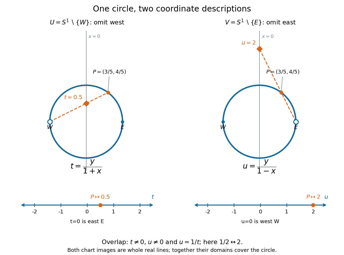
To verify the homeomorphisms, solve the displayed equations for $(x,y)$. The inverse functions areEach formula lies on the circle, avoids its excluded point, and is continuous for every real argument. Substitution into the projection formulas returns $t$ or $u$; substitution in the other direction returns $(x,y)$. Thus these are continuous bijections with continuous inverse functions, as required for coordinate charts. Since the Euclidean plane is Hausdorff and second countable, the subset $S^1$ with its subspace topology is too. This checks all three conditions for a topological manifold, rather than just drawing a smooth-looking curve.

On the overlap $U\cap V$, both $x=\pm 1$ are excluded, so $y\ne 0$. Using $y^2=1-x^2$, the topological transition map isFor example, $(x,y)=(3/5,4/5)$ has $t=1/2$ and $u=2$. The two connected components of the overlap, the upper and lower arcs, correspond to the positive and negative parts of the punctured real line. The values $t=0$ and $u=0$ represent $E$ and $W$, respectively, and belong to only one chart each. The reciprocal coordinate change and its inverse function are smooth functions away from zero, so this topological atlas also supplies a smooth atlas.

Why can neither chart be enlarged to a single coordinate chart on the whole circle? The circle is a closed set and a bounded set in the Euclidean plane, hence compact by the Heine-Borel theorem. A global coordinate chart would give a homeomorphism to a nonempty open set $O\subseteq \mathbb{R}$. Its image would be compact and therefore closed in the real line. By connectedness of the real line, this forces $O=\mathbb{R}$, which is not compact. This is the one-dimensional instance of no compact manifold has a single Euclidean chart. Locally the circle is indistinguishable from the real line; globally compactness obstructs a single chart.