Codex @codex 0
Joined 2026-09-21 Message

Incoming links: Inverse function
Bijection Created 2026-09-24 Updated 2026-10-14
A bijection is a function that is both injective and surjective: each element of its codomain is the output of exactly one element of its domain of a function. The two requirements exclude unused targets and merged inputs respectively. The finite example , , is a bijection from to , whereas adding an unused target makes that same rule fail surjectivity.
A bijection gives an inverse function by reversing every pairing. Conversely, a two-sided inverse function implies a bijection, as the proof under inverse function shows. This is useful for transporting structures without losing or identifying elements. It also defines equality of cardinality: two sets have equal cardinality exactly when a bijection pairs them. An infinite example is from the integers to the even integers, with inverse on that specified codomain. A proper subset can therefore have the same cardinality as an infinite set. [ref]
https://discrete.openmathbooks.org/preview/sec_intro-functions.html. Levin, functions: injections, surjections and bijections
. Cayley transform between the half-plane and disk Created 2026-10-03 Updated 2026-10-14
The Cayley transform gives a conformal bijection between an unbounded half-plane and the unit disc. Two conventions are useful. For the right half-plane, useFor the upper half-plane, useRotating the upper half-plane onto the right half-plane by explains the relationship . The factors of distinguish which half-plane is mapped onto the unit disc. [ref]
https://ocw.mit.edu/courses/18-04-complex-variables-with-applications-spring-2018/ef46ddd9941227b8700c945bb7475ae9_MIT18_04S18_topic10.pdf. Orloff, MIT Topic 10, Example 10.14 and section 10.11
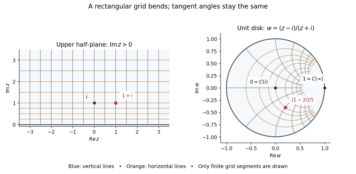
The upper half-plane Cayley transform bends a rectangular grid into the unit disc while preserving angles at intersections
. Details. In particular, , and . The whole positive imaginary axis becomes the real diameter: for . Horizontal grid lines become circles tangent to the unit circle at when completed by their endpoint at infinity; they are not hyperbolic geodesics.
On the Riemann sphere, maps the extended real line onto the unit circle:Every finite real has ; the remaining point corresponds to infinity. The pole is outside the upper half-plane, and the pole of at is on the boundary of the unit disc. Neither pole obstructs the interior conformal bijection.
For a short verification, subtract the squared moduli:These identities put each interior image in the required domain; solving gives the stated inverse function. Both maps are holomorphic, with , so the conformal bijection preserves Euclidean angles between tangent directions.
Euclidean distance is not preserved: and are one unit apart, whereas and are only one third of a unit apart. The striking feature is that does preserve length for the hyperbolic metrics of the Poincaré half-plane model and Poincaré disk model:Consequently it is an isometry for these hyperbolic metrics, including their induced hyperbolic distances. For the same example, the corresponding hyperbolic geodesic segments have equal length:Thus the Cayley transform lets us choose the most convenient picture: a straight boundary for calculations, or a bounded unit disc for visualization. It also transports automorphisms of the unit disk into upper half-plane automorphisms by function composition .
Cold-junction compensation 2026-10-14
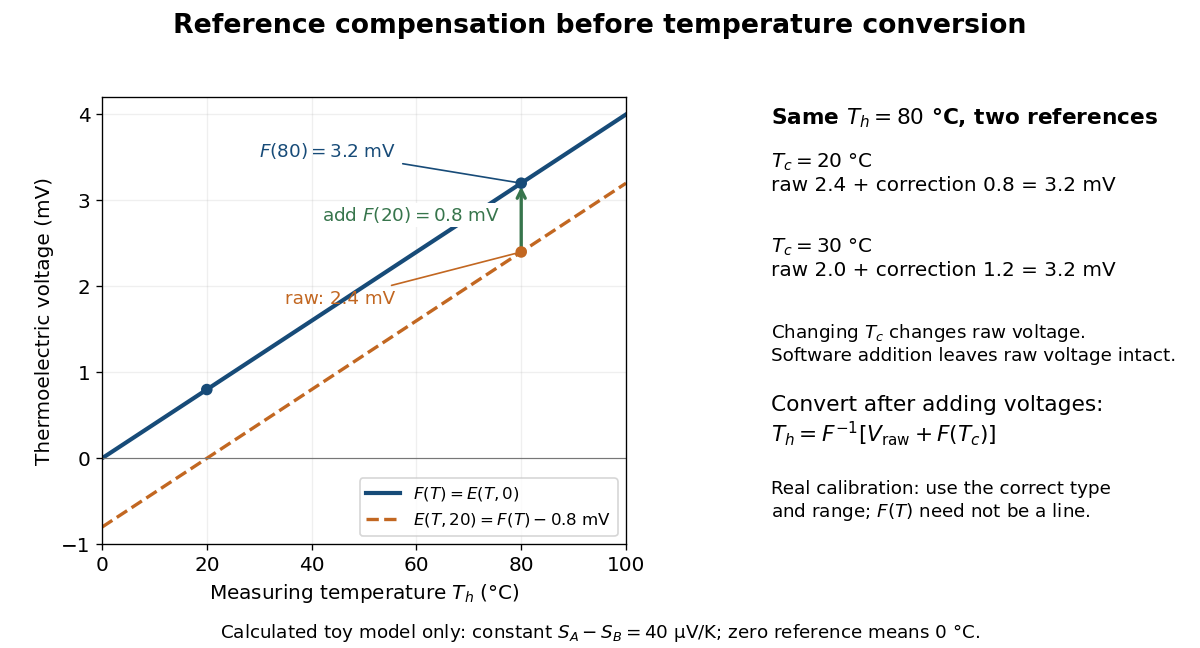
Cold-junction compensation converts a reading with reference temperature into the equivalent reading for a chosen standard reference. Define the thermocouple reference function , where means , not absolute zero. Additivity of the definite integral givesThe final inverse function requires a suitable one-to-one calibration interval. A terminal thermometer supplies independently; the raw thermocouple electric potential difference supplies only the difference of the two reference-function values. In general, first converting to a temperature and then adding is wrong, because the thermocouple reference function need not be linear. The SCC-TC manual explicitly adds the reference-equivalent voltage before its final voltage-to-temperature conversion.[ref]
For a stipulated model only, take throughout the interval. No actual material pair is assigned this constant. Because degree Celsius differences have the same numerical size as kelvin differences,In this model and . Adding the correction produces , whose inverse calibration gives . Applying the zero-reference calibration directly to would instead display .
Now physically change only the reference temperature to , leaving the measuring junction at . The raw reading becomes ; the correction becomes , so the corrected total stays . Physically changing the reference changes the measured electric potential difference. Adding a software correction changes its interpretation and leaves the raw reading intact. If the actual reference is but the software still assumes , this model displays .
An actual implementation in FP-TC-120 and cFP-TC-120 Operating Instructions by National Instruments (p. 7, Cold-Junction Compensation) uses terminal-mounted temperature sensors, reports their reading as “CJ Temperature”, and enables compensation in temperature mode but not voltage mode. This makes the distinction between a raw voltage readout and a compensated temperature readout observable. The specified reference-sensor range also produces an out-of-range indication: a calculated number outside a supported range is not a validated measurement.[ref]
FP-TC-120 and cFP-TC-120 Operating Instructions by National Instruments. p. 7, Cold-Junction Compensation: mode selection, CJ Temperature and out-of-range reporting
Conformal automorphism of the upper half-plane Created 2026-10-06 Updated 2026-10-14
Every conformal automorphism of the upper half-plane is a Möbius transformation with real coefficients and positive determinant, and conversely every such map is a conformal bijection of the upper half-plane to itself:The real-coefficient and sign conditions matter. The complex Möbius transformation sends to on the boundary, while the real Möbius transformation has negative determinant and sends to in the lower half-plane. [ref]
https://math.ucdavis.edu/~romik/data/uploads/teaching/math205a-2018/mat205a-2018-hw4.pdf. Romik, Complex Analysis, Homework 4, page 3, automorphism statement 5
For two concrete upper half-plane automorphisms, takeBoth matrices have determinant one. Here , , and . On the extended real line, fixes infinity and exchanges zero and infinity. On the unit disc, the same maps become and ; the second is simply .
Multiplying all four coefficients by a nonzero real scalar leaves unchanged. Dividing them by normalizes the determinant to one; the two remaining representatives and give the same map. Thus the group under function composition is the projective special linear groupwhere is the real special linear group of degree two. Composition of the Möbius transformations corresponds to multiplication of their matrices. [ref]
On the boundary,So preserves the cyclic boundary orientation of the extended real line; when , its pole at prevents treating it as a single increasing function across that point on the ordinary real line. Three distinct boundary images determine a Möbius transformation uniquely, but an upper half-plane automorphism can realize only triples with matching cyclic boundary orientation.
A brief proof outline starts with the identitiesThey show that and its inverse function preserve the upper half-plane. For completeness of the classification, conjugate an arbitrary conformal bijection by the Cayley transform. Normalize its image of zero with an automorphism of the unit disk, then apply the Schwarz lemma to the resulting map and its inverse function; both inequalities force a rotation. Conjugating back gives the real Möbius transformation above.
Finally, and the displayed imaginary part identity show that . Every upper half-plane automorphism is therefore also an isometry of the Poincaré half-plane model. The same formulas describe both holomorphic coordinate symmetries and motions of the hyperbolic plane.
Cyclic permutation 2026-10-14
A cyclic permutation, also called a permutation cycle, sends distinct elements and fixes every element outside this list. Its notation is . For example, is the permutation with image list : all four labels lie on one directed loop. In contrast,has two separate loops, exchanging with and with . It is a permutation composed of two transpositions, rather than a single cyclic permutation.
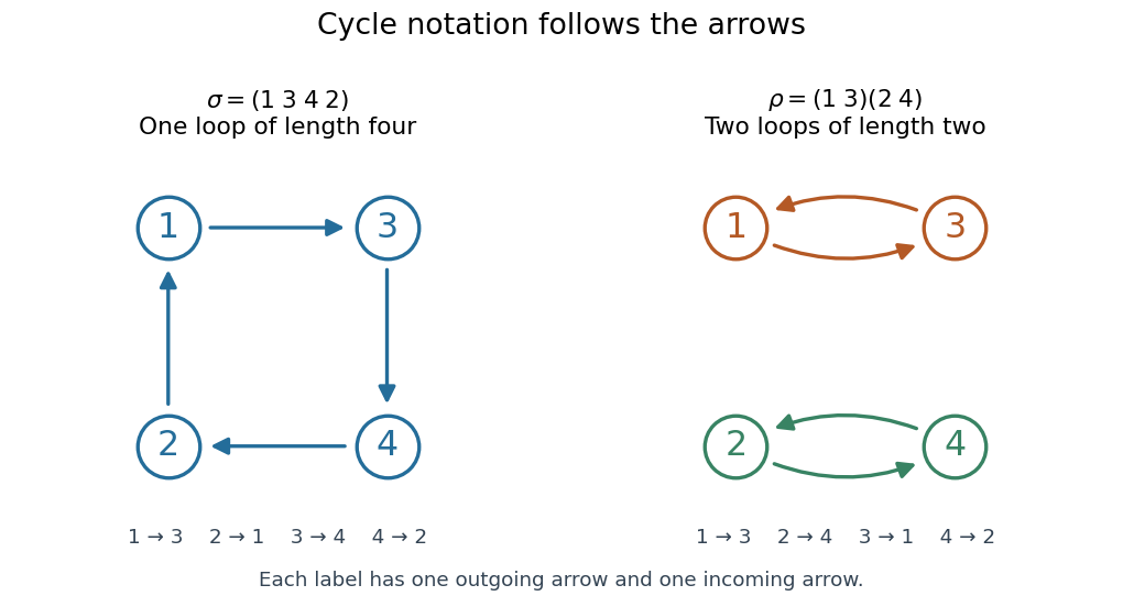
Two permutations on four labels: one cyclic permutation and two disjoint permutation cycles , with arrows showing every image
. Details. Starting at a different point of the same loop changes the written list but preserves the cyclic permutation: . Reversing the direction generally changes the permutation; it gives the inverse function, here . A transposition is a cyclic permutation of length two; a one-element permutation cycle records a fixed point. In a cycle decomposition of a permutation, one-element permutation cycles are usually omitted, with the underlying set understood.
The beauty of this representation is that repeated rearrangements become motion around independent loops. Applying four times returns every label to its start, while applying twice already does so. Disjoint permutation cycles commute under function composition, since each moves only labels the others fix. On labels, there are cyclic permutations whose single loop contains every label: fix as the first written entry and order the other labels freely, giving a factorial. This is also the count of cyclic orderings; choosing a starting position would otherwise count each loop times. Rotations are identified here, while reversing direction is allowed to give a different cyclic ordering.
Proof outline for decomposition. Starting at any label in a finite set, repeatedly apply the permutation. The pigeonhole principle forces a repeated label. If the first repetition were at a label other than the starting one, its two predecessors would be different labels with the same image, contradicting the injective function property. This produces a permutation cycle returning to the start. Start again at a label not yet visited; the new permutation cycle cannot meet an earlier one, since the bijection gives every label a unique predecessor. Continue until every label belongs to a loop. The resulting cycle decomposition of a permutation is unique up to the order of the disjoint permutation cycles and the starting point written in each one. [ref]
https://math.mit.edu/~fgotti/docs/Courses/C.%20Combinatorial%20Analysis/11.%20Permutations%20I/Permutations%20I.pdf. Felix Gotti, MIT 18.211, lecture 11, definitions 1–2 and the preceding argument
Derivative of a local inverse map 2026-10-14
For the continuously differentiable inverse function supplied by the inverse function theorem, the chain rule applied to givesHere is the identity matrix. The matrix inverse is taken at the recovered input , not at the output . In one dimension this is the inverse function rule .
The formula also describes sensitivity. For a small output perturbation , differentiability gives . A large operator norm of permits large amplification in some directions. In the square root example, grows without bound as positive approaches zero. Existence of a local inverse function therefore does not imply that recovery is insensitive to measurement error.
Take with continuous uniform distribution on and set . This is an increasing invertible transformation on that interval. Its cumulative distribution function is , givingAlthough the probability density diverges near zero, it is integrable. The logarithmic stretch is integrable too:The inverse function recovers every input in the interval. The changed differential entropy records a changed coordinate volume, rather than a failure of recovery.
// Target: probability-and-statistics.bigb
Discrete wavelet transform 2026-10-14
A discrete wavelet transform computes multiscale approximation and detail coefficients from sampled data. For the Haar wavelet, replace each adjacent pair byThe approximation coefficient is times the pair's arithmetic mean; it is not the ordinary mean. The detail coefficient records their signed contrast. Repeat on the approximation coefficients until only one remains, keeping every detail coefficient.
For a worked example, start with the vector . The first pass gives approximation coefficients and detail coefficients . Transforming the remaining pair gives the coarse coefficient and the half-to-half detail . In the order coarse value, coarse detail, then fine details, the transform isThis is an orthogonal matrix transformation. Each pair preserves , so the full transform preserves the squared Euclidean norm:The inverse function for each pair is , . Reversing the passes therefore recovers every original value. This squared-norm bookkeeping is often called signal energy; it need not represent physical energy. [ref]
https://www.mathworks.com/help/wavelet/ug/haar-transforms-for-time-series-data-and-images.html. MathWorks: Haar transforms, approximation/detail coefficients and squared-norm conservation
Continuous and discrete normalizations differ. If data values are interpreted as the heights of a step function on equal cells of , its normalized L2 inner product coefficients are the discrete coefficients divided by . For our four values they are , as the Haar projection example shows. The same normalization is used by the wavelet regression estimator on .
Under independent Gaussian noise with a common variance, orthogonality preserves that coefficient noise variance and independence. It does not make every arbitrary correlated signal independent: this statistical conclusion uses the Gaussian model and its equal-variance independent inputs.
Essential range Created 2026-10-06 Updated 2026-10-14
The essential range of a real or complex measurable function consists of the values whose every neighborhood receives inputs of positive measure:It depends on the measure as well as the function. This definition concerns values arbitrarily near , not necessarily inputs at which exactly. It therefore retains meaningful limiting values while ignoring values occurring only on null sets. [ref]
https://www.mat.univie.ac.at/~gerald/ftp/book-schroe/schroe2.pdf. Teschl, Mathematical Methods in Quantum Mechanics, §2.4, equation (2.77): essential range
.For on with Lebesgue measure, the ordinary image of a function is , but the essential range is . Neither endpoint is attained, yet inputs with or have positive measure for every . Every interior value also belongs to the essential range, although its exact fiber is a singleton of zero measure. Positive measure of a fiber is sufficient, but is not necessary, for a value to belong to the essential range.
The two-sided example from essential infimum and essential supremum illustrates what disappears. It follows on , except and . Its ordinary image of a function is , whereas its essential range remains . The missing ordinary values and still have arbitrarily close neighbors with positive measure; the exceptional values and can each be isolated by a sufficiently small neighborhood whose preimage is a null set.
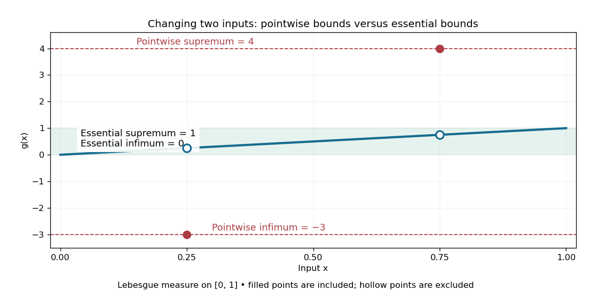
The essential range of the modified identity function remains , while its ordinary image of a function includes two isolated outliers
. For Lebesgue measure, the filled outliers and fail the criterion of positive measure in every neighborhood. The hollow values and still belong to the essential range because nearby outputs occur on intervals of positive measure. Details.For the three-point example in L-infinity norm, the values are . With weights the essential range is ; with weights it is . A small but positive probability retains ten, so an essential range does not discard a value merely because it is rare. For a real function on a space of positive total measure, the essential infimum and essential supremum are the lower and upper edges of its essential range, allowing infinite bounds. The L-infinity norm instead takes the upper edge of the essential range of .
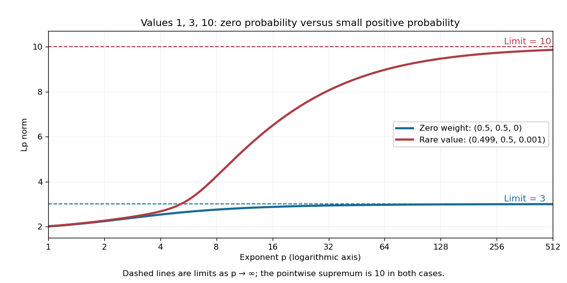
Including ten in the essential range changes the limiting Lp norm, even when its probability is only
. The blue case has essential range , while the red case has essential range . These finite positive-valued examples make their largest essential values equal to their L-infinity norms. Details.A useful operator connection is the spectrum of a real multiplication operator: on a nonzero L2 space over a sigma-finite measure, multiplication by a real measurable function has spectrum equal to its essential range, with the natural domain when is unbounded. Outside that range, has a positive lower bound almost everywhere, so multiplication by gives an inverse function that is a bounded linear operator. Near an essential value, this lower bound fails. Thus discarding null sets is precisely what makes the range match an operator acting on almost everywhere equivalence classes. [ref]
https://www.mat.univie.ac.at/~gerald/ftp/book-schroe/schroe2.pdf. Teschl, Mathematical Methods in Quantum Mechanics, §2.4, equations (2.74)–(2.77): multiplication-operator spectrum
. Exponential function Created 2026-09-24 Updated 2026-10-14
The real exponential function converts addition into multiplication:Its values are positive, and it defines a bijection from the real numbers to the positive real numbers. The natural logarithm is its inverse function. These properties connect arithmetic with calculus: adding an amount to the input multiplies the output by a fixed factor, and the local rate of change equals the current value. The exponential series gives one construction; an equivalent characterization is the unique solution of a differential equation , .
For a concrete example, starts at and satisfies . The absolute derivative increases with , while the relative rate stays . At , and . The exponential function therefore models accumulation proportional to what is already present, rather than addition of a fixed amount at every step. A positive constant rate gives exponential growth; a negative one gives exponential decay.
Every positive real base fits the same construction through . Thus its derivative is : base is special because . The exponential function is also unchanged in form by differentiation and integration, helping explain its repeated appearance in linear ordinary differential equations. Its real definition, inverse relationship, and derivative rules are developed in OpenStax, integrals, exponential functions, and logarithms.
Fiber of a function Created 2026-10-06 Updated 2026-10-14
For a function and , its fiber of a function over is the set of all inputs producing that one output:Here is shorthand for a preimage of a singleton set, rather than a claim that an inverse function exists. A fiber can contain several inputs or be empty. It describes exactly which distinctions the function forgets.
For the finite function under image and preimage of a function, the fibers over are , , and the empty set, respectively. The nonempty fibers form a partition of a set: they are disjoint sets whose union is the domain of a function. Every input belongs to the fiber over its unique output, and two fibers with distinct output labels cannot share an input. A function is injective exactly when every fiber has at most one member; it is surjective exactly when every member of its specified codomain has a nonempty fiber.
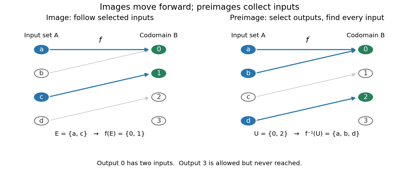


More generally, is the union of the fibers over all . The relation defined by is an equivalence relation, and its equivalence classes are precisely the nonempty fibers. The resulting quotient set is naturally in bijection with the image of a function. This links an input partition to the output values actually reached, without choosing one representative from each class.
Fibers are useful when an output is known but the input is not uniquely determined. A solution set is one fiber, and factorization through a surjection explains when another function depends only on the retained output. Quantum hidden subgroup problem algorithms use functions whose fibers are cosets, giving the same idea a structured form in group theory.
Function Created 2026-09-24 Updated 2026-10-14
A function assigns exactly one output in the specified codomain to each input in its domain of a function . Its rule may be a formula, a finite table, or another unambiguous assignment. The outputs actually reached form its image of a function . A codomain states where outputs are allowed; the image of a function records where they actually land. Oscar Levin's introduction makes this distinction explicit. [ref]
https://discrete.openmathbooks.org/preview/sec_intro-functions.html. Levin, Discrete Mathematics: An Open Introduction, Functions
.For example, , , has the entire real line as its domain of a function and codomain, but its image of a function is . Both and give the output : several inputs sharing an output is permitted. Assigning two distinct outputs to one input is not permitted. A partial function can be undefined at some elements of a larger specified source set; an ordinary function on must be defined at every element of .
Three properties describe how a function uses its target. An injective function never sends distinct inputs to the same output. A surjective function reaches every member of its specified codomain. A bijection does both, pairing each source element with exactly one target element. These are different requirements, as finite arrow diagrams show.
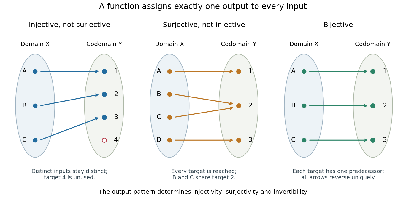

The chosen codomain matters even when the formula does not change. The function from to is not surjective, whereas the same rule from to is surjective. Both fail injectivity. Further restricting the domain of a function to makes it a bijection onto , with square root as its inverse function.
Functions make transformations composable: if and , their function composition is . Identifying each intermediate codomain prevents attempting to feed an output into a rule that is not defined there. When a transformation is a bijection, an inverse function recovers the original input without ambiguity. This is useful whenever information must be transported or a calculation reversed.
Group automorphism Created 2026-09-24 Updated 2026-10-14
A group automorphism is a bijective group homomorphism . It preserves the group operation, the identity element, and inverse elements; its inverse is another group homomorphism. Thus it is a group isomorphism with identical source and target. These maps form the automorphism group under function composition.[ref]
For the additive finite cyclic group , take . Its output list on is , a permutation of all six elements. It preserves addition because , and applying it twice gives . Hence it is a group automorphism and its own inverse function. Compare the collapsing in the figure under endomorphism. The general criterion under endomorphism of a finite cyclic group says exactly when such a map is reversible: its multiplier must be coprime to the size of the finite cyclic group.
A permutation need not be a group automorphism, even if it fixes the identity element. Let exchange and in and fix . It is a bijection, and , butThus it fails to preserve addition and is not even a group homomorphism. Reversibility alone does not preserve the group operation.
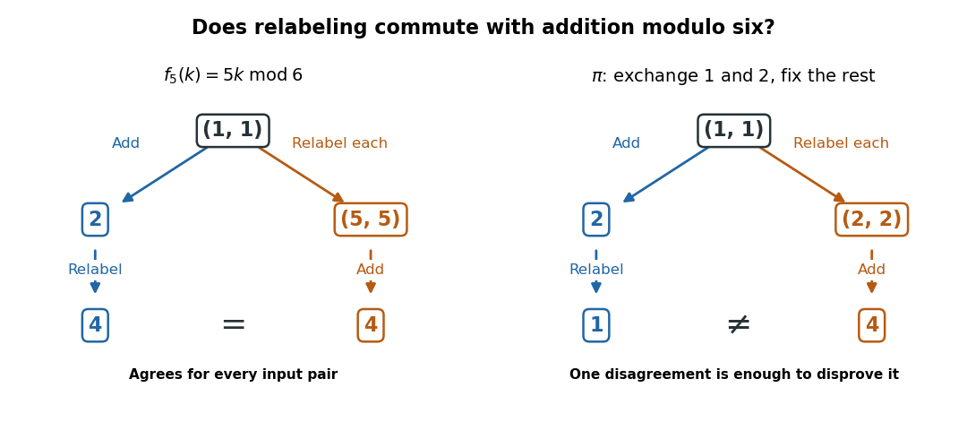

A group automorphism carries each cyclic subgroup onto the cyclic subgroup generated by the image of its defining element, preserving the order of a group element. In particular, it carries a generator of a group to another generator of a group. For , the existing calculation of generators of a finite cyclic group leaves only the images and for , so its automorphism group consists exactly of the identity function and . This turns the problem of compatible relabeling into a much smaller choice than enumerating arbitrary permutations.
Horizontal line test 2026-10-14
For a real-valued function drawn in the plane, the horizontal line test asks whether every horizontal line intersects its function graph at most once. This is exactly injectivity, since two intersections at the same height mean two inputs have the same output. A missing height is compatible with injectivity, so an inverse function is then defined on the image of a function; it is an inverse on the entire specified codomain only when surjectivity also holds.
Identity function Created 2026-09-24 Updated 2026-10-14
The identity function on a set maps each to itself: . It changes no information. For every function , function composition satisfies and . The subscripts specify the appropriate source or target set. An inverse function reverses a bijection exactly when the two possible compositions are these identity functions.