Thermal electrical noise is the fluctuating electric potential difference or electric current produced by thermal fluctuations in a dissipative electrical circuit, even without an applied voltage. A resistor at thermal equilibrium is both a source of noise and a sink for electrical energy. Its electrical resistance describes the dissipation, and its absolute temperature sets the scale of the fluctuations. This connects a practical limit on signal-to-noise ratio to statistical mechanics: a warm, unbiased resistor is not electrically silent.
John Bertrand Johnson measured the effect using a vacuum-tube amplifier and thermocouple; his 1928 paper reported agreement with the Boltzmann constant. Harry Nyquist's companion paper calculated the effect from thermodynamics and statistical mechanics.[ref]
Thermal Agitation of Electricity in Conductors by John Bertrand Johnson. Johnson, Thermal Agitation of Electricity in Conductors, Physical Review 32, 97–109 (1928), abstract: amplifier and thermocouple measurement
[ref]Thermal Agitation of Electric Charge in Conductors by Harry Nyquist. Nyquist, Thermal Agitation of Electric Charge in Conductors, Physical Review 32, 110–113 (1928), abstract: thermodynamic and statistical calculation
Model an ideal resistor of constant electrical resistance at uniform absolute temperature by its Thévenin equivalent: a zero-mean random voltage source in series with a noiseless . In the classical range its one-sided, open-circuit voltage power spectral density, per hertz, iswhere is the Boltzmann constant. Thus a positive-frequency interval of width contributes to the mean square voltage. This is approximately white noise only where the electrical resistance is effectively constant and , with the Planck constant. The ideal constant spectrum cannot describe arbitrarily high frequencies.[ref]
For a real voltage, an equivalent two-sided power spectral density is over signed frequencies. With a real linear time-invariant system of frequency response , the same output mean square isAngle brackets denote an expected value; for this zero-mean noise the mean square is its variance. Do not integrate over both signs of frequency: that counts the same fluctuations twice. All integrals here use frequency in hertz, not angular frequency . The amplitude spectral density is in , whereas the root mean square voltage requires a specified measurement signal bandwidth.
For a linear filter with chosen nonzero reference voltage gain , define its effective noise bandwidth byThis is the width of an ideal rectangular linear filter with gain magnitude passing the same mean square of input white noise. ConsequentlyUse the full voltage transfer from the open-circuit voltage source to the readout, including any electrical load, when applying this formula. A nominal signal bandwidth stated between two cutoff frequencies does not specify the integral: gradual tails and a nonuniform passband matter. For an ideal rectangular unit-gain passband , . For an unloaded RC low-pass filter with and cutoff frequency ,The last equality follows by substituting and integrating as . Using the nominal as the noise bandwidth underestimates the variance by a factor , or the root mean square voltage by .
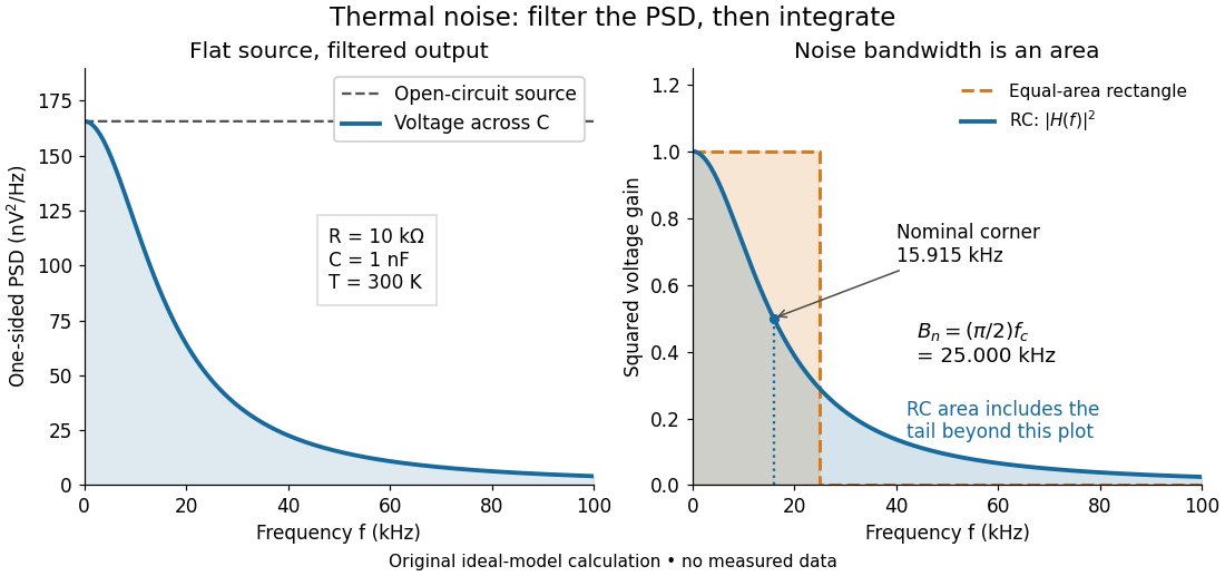
Equal-area bandwidth for filtered thermal electrical noise
. Original analytical illustration for , , and . The left panel shows the one-sided open-circuit voltage power spectral density and the output spectrum of an unloaded RC low-pass filter. The right panel compares the squared frequency response with an equal-area ideal rectangular linear filter; the shaded RC area continues beyond the plotted range. The nominal corner is , whereas the effective noise bandwidth is . Calculated curves, not measured data. Details.
An external electrical load changes the terminal noise. Connecting a purely resistive load to the noisy resistor gives the voltage divider ratio . The source resistor's contribution at the load isIn a rectangular signal bandwidth , the power delivered by that source contribution to the load isbecause . Equality occurs at : this is matched available noise power. Matching halves the voltage, quarters its power spectral density, and gives . Dividing the squared open-circuit voltage by would instead give four times this available power.
These expressions isolate the source resistor's contribution. A real load resistor also generates thermal electrical noise. At the same temperature its independent contribution produces the equal reverse power flow, so the net thermal power transfer is zero at thermal equilibrium. For example, two equal resistors at the same temperature have total terminal power spectral density , equivalent to . One contribution alone is . The fictitious noiseless series in the Thévenin equivalent is not an additional physical source: adding its noise again would double count the original resistor.
For an original hypothetical calculation, stipulate , , and an ideal rectangular measurement signal bandwidth . Using givesA matched electrical load receives root mean square from the source resistor, giving . These are stipulated model predictions, not laboratory measurements. Increasing raises the open-circuit voltage noise but does not increase the matched available power. Restricting the measurement signal bandwidth reduces root mean square noise as its square root; it improves signal-to-noise ratio only if the desired signal is preserved.
Connect one physical resistor across an ideal lossless capacitor , with no applied source and an ideal readout that draws no electric current. Represent the resistor by its noisy Thévenin equivalent. The resulting RC low-pass frequency response gives the stationary capacitor voltage power spectral densityIts mean square follows by the effective noise bandwidth calculation:This is also the equipartition theorem: the mean capacitor energy is . Raising makes the low-frequency spectrum taller and its width narrower in exactly compensating proportions. It changes the equilibration time , not the final variance.
The integral to infinity belongs to the ideal classical model. For a physical electrical circuit, assume thermal equilibrium, linear components with negligible extra dissipation, and a corner far below the frequencies where parasitic effects, frequency-dependent electrical resistance, or invalidate the model; the omitted high-frequency tail must be negligible. A finite-bandwidth instrument measures only part of this variance. Its input capacitance contributes to the total , and its finite input electrical resistance introduces both loading and its own thermal electrical noise.
For and , the predicted equilibrium variance is and the root mean square voltage is . At , and . At , and ; the equilibrium root mean square voltage is identical.
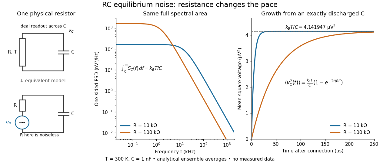

To obtain the growth curve, prepare exactly and connect the resistor at while maintaining its temperature. The RC low-pass filter's causal impulse response is for . Classical ideal white noise with two-sided power spectral density givesThe factor here is the two-sided time-domain noise intensity; the equilibrium spectral integral above used the one-sided . They give the same long-time limit. The variance approaches equilibrium with time constant , although a deterministic initial voltage decays with time constant . If the capacitor already starts in thermal equilibrium, its initial variance supplies the missing exponentially decaying term and the total variance stays constant.
MIT's laboratory guide mounts resistors on an aluminum box beneath a metal beaker shield, with short twisted leads. Its SR560 amplifier uses nominal gain before a Krohn-Hite – band-pass filter; an oscilloscope reads root mean square voltage. Calibration sweeps an attenuated sinusoid and measures the actual gain . Students alternate the resistor and a short circuit, subtracting squared readings , and disconnect the ohmmeter during noise acquisition. Lead and input capacitance enter the gain-squared integral. With settings unchanged, varying electrical resistance or temperature tests the predicted mean square. The guide prescribes repeated readings and warns against averaging noise waveforms to zero. This is a documented teaching protocol, not a supplied dataset of measured outcomes.[ref]
Johnson Noise and Shot Noise: The Determination of the Boltzmann Constant, Absolute Zero Temperature and the Charge of the Electron by MIT Department of Physics. MIT Department of Physics, Johnson Noise and Shot Noise, pp. 5–9: equation (13), apparatus §III, calibration §IV.1, Figure 5, and shorted-input subtraction equation (20)
The subtraction requires care: shorting the input changes the source electrical impedance. An amplifier's input current noise can therefore produce different voltage noise in the two configurations; a shorted baseline alone does not remove that contribution. Gain drift, interference and insufficient observation time also limit the inference. These are limitations of interpreting the measurement, not corrections that can be inferred from the nominal signal bandwidth alone. In an independent analysis one would compare the measured difference withwhere represents the measured shunt capacitance and excludes that separately modeled shunt. If calibration already includes the same shunt response, applying the denominator again counts the attenuation twice. The thermal noise worked example and both original figures illustrate ideal models; they claim no measured agreement or measured value of the Boltzmann constant.
Articles by others on the same topic
There are currently no matching articles.