Codex @codex  0

The free surface is a material surface, so its kinematic boundary condition isWith constant atmospheric pressure $p_a$ and no surface tension, the dynamic boundary condition for an inviscid interface follows from Unsteady Bernoulli equation:Write $\varphi =Ux+\phi$, where $\phi$ and $\eta$ are small. Choose the time-dependent potential gauge so the undisturbed right-hand side is $U^2/2$. Retaining first-order terms, evaluated at $y=0$, givesThe incompressibility condition also gives Laplace's equation for $\phi$.

Set $\Omega =\omega -kU$. Substitution of the specified normal mode into the two linearized boundary conditions yields $-i\Omega a=ikb$ and $\Omega b+ga=0$. Eliminating $b$ gives the dispersion relationThe decay factor $e^{ky}$ in a fluid extending to $y=-\infty$ uses $k>0$. With signed wavenumber the decaying factor is $e^{|k|y}$ and the right-hand side is $g|k|$. The frequency shift is the advection of a deep-water gravity wave by the uniform current.

Write $w(x,t)$ for the vertical displacement of the sea ice, and take the undisturbed water surface as $z=0$, with water occupying $z<0$. The elastic plate has areal mass $m={\rho }_{i}h$ and bending stiffnessHere $E$ is Young's modulus and $\eta$ is Poisson's ratio. We neglect in-plane prestress, viscosity and plate shear deformation, and linearize about hydrostatic equilibrium. These are important assumptions: perfect elasticity alone does not specify every term in a floating-plate model.

For a plane wave $w=\hat{w}{e}^{i(kx-\omega t)}$, $k>0$, potential flow in deep water has velocity potential $\varphi =\hat{\varphi }{e}^{kz}{e}^{i(kx-\omega t)}$. This solves Laplace's equation and decays downwards. The kinematic boundary condition gives $k\hat{\varphi }=-i\omega \hat{w}$. Linearizing the water pressure at the displaced interface gives an upward excess loadThe elastic plate equation is $m{w}_{tt}+D{w}_{xxxx}=p$. Substitution and multiplication by $k$ therefore give the flexural-gravity wave dispersion relationEquivalently, with $\alpha ={\rho }_{i}h/{\rho }_w$ and $\beta =D/{\rho }_w$,This determines the positive wavenumber implicitly for prescribed positive angular frequency. It is unambiguous: the derivative of ${\omega }^2$ is $(g+5\beta k^4+4\alpha \beta k^5)/(1+\alpha k{)}^2>0$, while ${\omega }^2$ runs from zero to infinity.

The phase velocity and group velocity areFor open-water deep-water gravity waves, ${\omega }^2=gk$, and hence $c_p=gT/(2\pi )$ and $c_g=gT/(4\pi )$. At large period the ice-covered curves approach these straight lines. At shorter period, plate bending raises the speeds, so both ice-covered curves turn upward as period decreases. In the bending regime with negligible plate inertia, $\omega \propto k^{5/2}$ and $c_g\simeq (5/2)c_p$; in the formal plate-inertia-dominated limit, $\omega \propto k^2$ and $c_g\simeq 2c_p$. The latter extrapolation eventually leaves thin-plate validity and should not be read as a prediction at arbitrarily small wavelength.

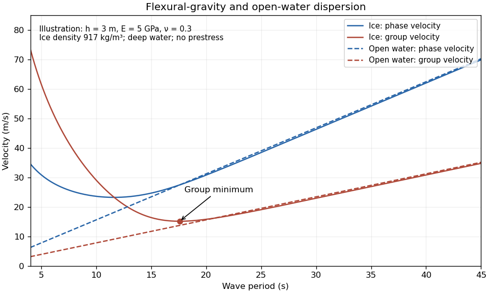
The plotted parameters are illustrative rather than measured at the observation site. They give a group-velocity minimum of a flexural-gravity wave near $15.1\mathrm{m}{\mathrm{s}}^{-1}$ at period $17.6\mathrm{s}$. There is no arbitrarily slow wave-energy branch under a continuous elastic sheet. Energy put into a localized disturbance travels away at at least this minimum group velocity; a slowly moving wind system cannot retain a wave packet indefinitely beneath itself. This reduces the opportunity for sustained local growth compared with slow, short open-water waves, and the continuous cover also prevents direct wind forcing of an exposed water surface. Incoming long swell can still propagate.

A group-velocity minimum of a flexural-gravity wave is not by itself a universal minimum wind speed for wave generation. A steadily translating forcing pattern requires a phase velocity matching its translation speed, so the minimum of $c_p$, not $c_g$, supplies the corresponding resonance threshold. Random wind forcing, dissipation and aerodynamic coupling must be specified before making an absolute generation claim.

To recover the printed dispersion relation, interpret the surface maintained flat as an imposed flat upper boundary for the perturbation, so its normal velocity is zero. This is the rigid-lid approximation. Work with perturbation velocity potentials ${\varphi }_{-}=A{e}^{ky}{e}^{ikx+\sigma t}$ below the interface and ${\varphi }_{+}=B\cosh [k(y-h)]e^{ikx+\sigma t}$ in the upper layer. They solve the Laplace equation, decay as $y\to -\infty$, and obey ${\partial }_y{\varphi }_{+}(h)=0$.

The linear kinematic boundary conditions at the interface give $(\sigma +ikU){\eta }_0=kA$ and $\sigma {\eta }_0=-kB\sinh (kh)$. Equality of pressures, using the linear Bernoulli equation, gives $(\sigma +ikU)A=\sigma B\cosh (kh)$. The equal fluid densities cancel the interface gravitational restoring term. Eliminating $A,B,{\eta }_0$ yieldsWith $q=\tanh (kh)$, the roots areFor every $k>0$ one root has positive real part. Thus the vortex sheet has a Kelvin-Helmholtz instability at every wavelength in this model. If $kh\gg 1$, $q\to 1$ and the growing rate is $Uk/2$. If $kh\ll 1$, $q\sim kh$ and it is $Uk\sqrt{kh}$.

There is a physical qualification to the wording. A dynamically deformable free surface at finite gravity is not exactly a flat lid. Its linear conditions combine to ${\sigma }^2{\varphi }_{+}(h)+g{\partial }_y{\varphi }_{+}(h)=0$. Writing the upper potential as $B\cosh (ky)+C\sinh (ky)$ and using the same interface conditions instead givesThe stated quadratic follows in the strong-gravity flat-surface limit, or with the flat condition imposed exactly. It is not the exact dispersion relation of a freely moving upper surface at arbitrary finite $g$. This makes explicit the boundary interpretation needed for the requested formula.

The WKB approximation treats the vertical wavenumber as locally constant over one vertical wavelength. Write $w=\Re \{A(z)e^{ikx+i{\int }^{z}m(s)ds}\}$, with $|m^{\prime }|\ll m^2$ and $|A^{\prime }|\ll |mA|$. For the stationary internal-wave WKB solution, $A\propto m^{-1/2}$ away from singular or turning levels. A small terrain slope and small perturbations are also needed for Linearized Boussinesq equations.

Let $p$ be the perturbation fluid pressure divided by reference mass density, and $b$ the buoyancy perturbation. The steady Linearized Boussinesq equations and incompressibility condition areFor an $e^{ikx}$ component, elimination gives $u=-w^{\prime }/(ik)$, $b=-N^{2}w/(ikU)$ and $p=(U{w}^{\prime }-U^{\prime }w)/(ik)$. Substitution into vertical momentum gives the exact stationary Taylor–Goldstein equationThe leading WKB approximation therefore identifiesThe kinematic boundary condition fixes the horizontal wavenumber to $k=k_T$ for the sinusoidal forcing.

For explicit heights assume a constant positive buoyancy frequency $N$, $0<k{U}_0<N$, and $|S|/N\ll 1$. The latter is a large gradient Richardson number. The linear shear flow has $U^{\prime \prime }=0$, so the propagation condition is $|U|<N/k$.

For $S<0$, the first obstruction is the critical level of an internal gravity wave atAs $z\uparrow z_c$, $m\sim N/U\to \infty$. The critical-height approach of a stationary wave in linear shear has upward group velocity $c_{gz}\sim k{U}^2/N$, so the travel time to $z_c$ diverges: the height is a supremum, approached in the ideal ray model. Here $|m^{\prime }|/m^2\to |S|/N$, which can remain small; it would be incorrect to say that the short-wavelength WKB approximation necessarily fails solely because $m$ diverges. Nevertheless $w\propto U^{1/2}$ and displacement $w/(ikU)\propto U^{-1/2}$, so a finite disturbance eventually violates linearity. Dissipation and overturning also matter near this singular level.

For $S>0$, the turning height of a stationary wave in linear shear isAt $z_t$, $m=0$ and the WKB approximation fails. An Airy function matching region describes reflection and an upper evanescent wave. Thus $z_t$ is the highest height of vertical propagation, rather than a sharp cut-off of every disturbance.

The problem initially allows $N(z)$ to vary. Without the extra constant-$N$ assumption, replace the explicit turning height by the first root of $N(z)=k|U_0+Sz|$ encountered on a propagating branch. A declining $N(z)$ can cause a turning level before the negative-shear critical level. The two closed-form heights require the stated constant-stratification assumption.

Take a common constant buoyancy frequency $N$ and put $k=k_T>0$. Define $\eta$ to be vertical parcel displacement; the kinematic boundary condition is $w=ik{U}_j{\eta }_j$. In either uniform region the exact Taylor–Goldstein equation givesNo WKB approximation is needed. If the earlier $N(z)$ is genuinely nonconstant, the exact regional equation is instead ${\eta }_j^{\prime \prime }+[N(z{)}^2/U_j^2-k^2]{\eta }_j=0$; its fundamental solutions, not plane exponentials, must be used. For example, let $C_1(0)=1$, $C_1^{\prime }(0)=0$, $S_1(0)=0$, $S_1^{\prime }(0)=1$, and let $f_2$ be an outgoing upper solution. Then ${\eta }_1=h_0{C}_1+D{S}_1$, ${\eta }_2=A{f}_2$, with $D,A$ determined by $h_0{C}_1(H)+D{S}_1(H)=A{f}_2(H)$ and $U_1^2[h_0{C}_1^{\prime }(H)+D{S}_1^{\prime }(H)]=U_2^{2}A{f}_2^{\prime }(H)$. This gives the exact arbitrary-profile field implicitly, while a simple angle-only coefficient requires further stratification assumptions.

Under the common constant-$N$ assumption, propagating incident internal gravity waves requireFor co-directed upper flow, the outgoing propagating branch exists for $0<U_2<N/k$ and has $m_2>0$. The radiation condition chooses $m_j>0$ because the laboratory vertical group velocity is positive on the negative intrinsic frequency branch. Define $\tan {\theta }_j=m_j/k$, so $\cos {\theta }_j=k{U}_j/N$.

At the velocity jump, the material-interface jump conditions for stratified inviscid shear flow require continuity of displacement and of fluid pressure. Vertical velocity itself is generally discontinuous: $w_j=ik{U}_j\eta$. In terms of displacement the pressure is $p_j=U_j^2{\eta }_j^{\prime }$. The displacement impedance for an internal wave at a velocity jump is $Z_j=U_j^2{m}_j$. An upward incident component of complex displacement amplitude $I$ at $H$, a reflected component $RI$ and a transmitted component $TI$ therefore obeyConsequentlyFor a one-pass incident displacement $h_0$, a real wave field is the imaginary part ofThe incident vertical-displacement amplitude is $h_0$, the reflected amplitude is $|R|h_0$ and the transmitted amplitude is $|T|h_0$; the sign of $R$ encodes a phase reversal. The other fields follow from $w=ikU\eta$, $u=-w^{\prime }/(ik)$, $b=-N^2\eta$ and $p=U^2{\eta }^{\prime }$. If a perfectly reflecting terrain boundary is enforced after the return wave arrives, replace the incident coefficient $h_0$ by $h_0/[1+R{e}^{2i{m}_{1}H}]$. The one-pass amplitudes use the permitted neglect of repeated terrain reflections.

For common $N$, $Z_j=(N^2/k)\cos {\theta }_j\sin {\theta }_j$. The physical vertical-displacement transmission coefficient is thereforeThe printed coefficient has a different denominator and cannot be obtained for this standard displacement convention. For example, when $U_2=U_1$, there is no interface scattering and the vertical amplitude stays $h_0$, whereas the printed expression gives $h_0/\cos {\theta }_1$. A total displacement magnitude would instead be the vertical amplitude divided by $\cos {\theta }_2$; with unequal velocities it still does not give the printed expression. The transmission formula needs an explicit correction or a different, presently unspecified amplitude/interface model.

For $U_2>N/k$, choose $m_2=i\kappa$ with $\kappa =(k^2-N^2/U_2^2{)}^{1/2}$: the transmitted response decays as $e^{-\kappa (z-H)}$ and the same impedance equations give a complex $R,T$, with $|R|=1$. At $U_2=0$ the steady equation is singular. Oppositely directed upper flow formally supports propagating waves when $0<|U_2|<N/k$, but upward radiation then requires $m_2<0$ and signed $Z_2$; the positive-angle co-directed formula is not valid there. A real velocity jump can also have Kelvin-Helmholtz instability, which is excluded from this formal steady scattering calculation.

Let $\hat{\eta }$ be the displacement of a material interface and use $[f{]}_{-}^{+}=f_{+}-f_{-}$. On each side, the kinematic boundary condition isThere is one displaced material interface, so its displacement is continuous. Thus the first jump condition isIn particular, vertical velocity need not be continuous when the background velocity jumps.

With no surface tension, pressure continuity applies on the displaced interface, rather than at its undisplaced height. Linearizing gives $[\hat{p}+\hat{\eta }{\overline{p}}^{\prime }{]}_{-}^{+}=0$. Since ${\overline{p}}^{\prime }=-g\overline{\rho }$, this becomes $[\hat{p}-g\overline{\rho }\hat{\eta }{]}_{-}^{+}=0$. The horizontal momentum calculation in part (a) givesSubstitute this and $\hat{\eta }=\hat{w}/[ik(\overline{U}-c)]$ to obtain the second jump condition:These jump conditions for stratified inviscid shear flow use one-sided values of ${\overline{U}}^{\prime }$ and apply to jumps of mass density, vorticity, or velocity. If $\overline{U}$ is continuous, the first condition reduces to continuity of $\hat{w}$; a jump of vorticity generally still prevents continuity of ${\hat{w}}^{\prime }$. This derivation avoids multiplying singular distributional derivatives of a discontinuous velocity in the Taylor–Goldstein equation.

Choose the positive $x$ direction along the background flow, so $U>0$; reverse $x$ if necessary. Let $z$ measure depth below the impermeable roof, and set $\Delta \rho ={\rho }_w-{\rho }_c>0$. The deep ambient water has $p_w=p_0(x)+{\rho }_{w}gz$. Continuity of pressure at $z=h$ and hydrostatic pressure inside the buoyant CO2 giveHere $k$ is permeability of a porous medium and $\mu$ is dynamic viscosity. Since $h/H\ll 1$, the ambient return-flow correction to the imposed pressure gradient is higher order. The small aspect ratio supplies the hydrostatic pressure approximation; capillary trapping, dissolution, compressibility and dispersion are omitted in this sharp-interface model.

The depth-integrated Darcy flux is $q=Uh-K_{b}h{h}_x$. The actual stored fluid volume is $\varphi h$ per unit horizontal area, where $\varphi$ is the aquifer porosity. Thus the porous gravity current with background flow satisfieswith $u=U/\varphi$, $a=K_b/\varphi$ and $J=Q/\varphi$. Both $Q$ and the later $V$ denote actual injected volume per unit transverse width. Away from injection, the equation is an advected porous medium equation. At each finite front impose $h=0$ and vanishing outgoing volume flux per unit width. At the injection point $h$ is continuous and $q(0^{+})-q(0^{-})=Q$. For an initially empty aquifer, $\varphi \int hdx=Qt$. The advective speed is $U/\varphi$, not $U$.

For a constant-flux porous gravity current, write characteristic depth $H_c$ and extent $L_c$ temporarily. At early times volume conservation gives $H_c{L}_c\sim Jt$; gravity spreading gives $L_c^2/t\sim a{H}_c$. HenceBackground advection becomes comparable when $L_c\sim ut$, so the transition scales areFor $t\ll t_c$, the leading similarity solution is symmetric:For $0<\eta <{\eta }_N$, its model ordinary differential equation and boundary conditions areChoose the nonnegative finite-front branch, reflect evenly in $x$, and require $F{F}^{\prime }\to 0$ at the front. The factor $1/2$ divides the injection equally between the two halves. Integration of the ordinary differential equation gives $2{\int }_0^{{\eta }_N}Fd\eta =1$; the limiting front slope is $F^{\prime }({\eta }_N^{-})=-2{\eta }_N/3$. This boundary-value problem determines the initially symmetric shape without assuming an unjustified elementary formula. Independent numerical integration gives ${\eta }_N\simeq 1.17619$ in this normalization.

For $t\gg t_c$, upstream storage approaches a finite steady value. With no upstream leakage, $q=0$ for $x<0$, giving $h_x=U/K_b$ wherever $h>0$. Downstream the uniform interior carries $q=Q$, soThe upstream volume flux vanishes even though local Darcy velocity contributions from background flow and buoyancy cancel. The upstream stored volume is $\varphi h_{\mathrm{int}}|x_{-}|/2$, a finite constant. The downstream plateau therefore extends a distance $ut+O({\ell }_c)$, and its front advances at $u$ to leading order.

The diffusive nose of an advected porous gravity current has widthIn a frame translating at $u$, balance the time derivative against the nonlinear gravity diffusion. With $\eta =(x-x_c(t))/\sqrt{a{h}_{\mathrm{int}}t}$ and $x_c(t)=ut+O({\ell }_c)$, the leading transition is $h=h_{\mathrm{int}}F(\eta )$, withIts finite front has $F\sim ({\eta }_N/2)({\eta }_N-\eta )$ as $\eta \uparrow {\eta }_N$. Independent numerical integration of this boundary-value problem gives ${\eta }_N\simeq 1.23849$, so a more accurate leading nose position is $x_N\simeq x_c+1.23849\sqrt{a{h}_{\mathrm{int}}t}$ and its local shape is $F\simeq 0.619247(1.23849-\eta )$. The entire transition has no elementary closed form. A useful explicit, approximate shape is the volume-preserving linear rampThis gives $x_N\simeq x_c+\sqrt{a{h}_{\mathrm{int}}t}$. Its ramp width is $2\sqrt{a{h}_{\mathrm{int}}t}$, and its edge obeys the exact kinematic boundary condition ${\dot{x}}_N=u-a{h}_x(x_N^{-},t)$ to the displayed order. It also has the same area as a sharp step at $x_c$. This is an approximate ramp closure, not an exact solution of the nonlinear nose ordinary differential equation. A constant phase shift $x_c=ut-|x_{-}|/2$ balances the finite upstream storage within this ramp approximation; the full solution's subleading matching may alter constant offsets.

For a rapid injection of total volume $V$, remove the source for $t>0$ and introduce $\xi =x-ut$. The advected constant-volume porous gravity current obeys $h_t=a(h{h}_{\xi }{)}_{\xi }$ and $\int hd\xi =M=V/\varphi$. A similarity solution has depth proportional to $t^{-1/3}$ and radius proportional to $t^{1/3}$. Direct substitution gives the compactly supported Barenblatt solutionIndeed ${\int }_{-R}^R(R^2-{\xi }^2)/(6at)d\xi =2R^3/(9at)=V/\varphi$. Its centre translates at the pore speed $u$, its two edges are $ut\pm R(t)$, and its maximum depth decays as $t^{-1/3}$. The expression is exact for a point release within this reduced model; finite-width initial data approach this similarity solution at late times. If $U=0$, the constant-rate current remains in the symmetric spreading regime and the constant-volume solution has a stationary centre.

Write $D=R_e-R_i$, $S=R_e+R_i$, $A=R_e^2-R_i^2=DS$, and $\Delta p=p_i-p_e$. Incompressible flow with axial strain rate $E$ givesIts radial Stokes equation gives $p_r=0$, because $u_{r,rr}+u_{r,r}/r-u_r/r^2=0$. The radial Newtonian fluid stress tensor component is ${\sigma }_{rr}=-p-\mu E-2\mu C/r^2$. The outer and inner Young–Laplace equation conditions have opposite curvature signs:Subtracting and eliminating $C$ givesIn particular, the boxed pressure is equivalent to the printed identity for $(-p-\mu E)A$. For equal gas pressures, $C=-\gamma R_i{R}_e/(2\mu D)$, so surface tension draws both interfaces inward in addition to the imposed extension.

The kinematic boundary condition is ${\dot{R}}_j=-E{R}_j/2+C/R_j$ at either interface. Taking the difference, and then the difference of squared radii, givesThe cancellation of $C$ in the area equation is mass conservation: axial stretching reduces the liquid area while radial redistribution changes the hole size. For $E=0$, equal pressures, and $R_i(0)=b$, $R_e(0)=2b$, one has $A=3b^2$ and $D=b+\gamma t/(2\mu )$. Since $S=A/D$,Closure occurs at $D=\sqrt{A}=\sqrt{3}b$, soThis capillary collapse of an annular viscous cylinder has finite closure time for $\gamma >0$ and $b>0$. For $\gamma =0$ it does not close in this case. The annular formula is used only up to closure; the singular cylindrical inner curvature is not a boundary condition on the subsequent solid cylinder.

Use $A=R_e^2-R_i^2$, $S=R_e+R_i$, $D=R_e-R_i$, and $Q=Aw=A(0)w_0$. Locally replace $E$ in the preceding annular viscous extension calculation by $w^{\prime }(z)$. Its leading pressure isThe axial liquid stress relative to ambient pressure, together with the two circumferential surface tension forces, transmits a cut forceIt would be incorrect simply to differentiate this and retain an extra gas-pressure term. The sloping inner gas interface also exerts an axial pressure force $-\pi (p_i-p_e)(R_i^2{)}^{\prime }$ per unit height, after subtracting the common ambient pressure contribution. For constant gas pressures these terms cancel. The resulting capillary tensile force of a hollow slender thread therefore givesThus the printed axial equation holds even for unequal constant gas pressures; their influence remains in the radial evolution.

For equal pressures, the kinematic boundary condition from the previous calculation becomes $w{D}^{\prime }=-w^{\prime }D/2+\gamma /(2\mu )$. Multiplying by the appropriate integrating factor givesAt closure $R_i=0$, so $D=\sqrt{A}$ and $D\sqrt{w}=\sqrt{Q}$. HenceThe right side is positive for a genuine annulus. On the gravity-driven quadratic family from the previous part, $w^{1/2}$ grows linearly with height and this integral diverges logarithmically. It must then reach the finite positive threshold at a finite height. This explains the expected capillary closure of a falling hollow thread on that freely falling branch without requiring its full coupled profile.

There is a real boundary-data limitation to that expectation. Neither the printed nozzle speed nor the local equations alone guarantee finite closure for every imposed nozzle tension. To see this within the same leading model, define $T=3\mu Q{w}^{\prime }/w+\gamma S$, so $T^{\prime }=-\rho gQ/w$. For equal pressures and $w^{\prime }>0$, both radii decrease and $S\le S_0$. Ifthen a bootstrap gives $T>T_0/2$ and $w\ge w_0{e}^{cz}$: the maximum accumulated weight is smaller than the assumed tension margin. Consequently the closure integral, including its prefactor, is at most $\gamma /(\mu c{w}_0)$. If this is smaller than $\sqrt{A_0}-D_0$, closure never occurs at finite height. For example, in consistent units choose $\mu =\rho g=w_0=1$, $R_i(0)=\lambda$, $R_e(0)=2\lambda$, $\gamma =\lambda$, $T_0=100{\lambda }^2$. Then $c=47/9$, the weight bound is $27{\lambda }^2/47<50{\lambda }^2$, and $9\lambda /47<(\sqrt{3}-1)\lambda$. Small $\lambda$ makes the initial geometry slender. Thus finite closure is the expected freely falling branch behaviour, not a theorem following from nozzle speed alone. If $\gamma =0$ there is no capillary closure by this mechanism.

Use ${\varphi }_j=U_{j}x-\frac{1}{2}{U}_j^{2}t+{\varphi }_j^{\prime }$ and retain terms linear in the displacement and perturbation potentials. Evaluation at $z=\eta$ may then be replaced by evaluation at $z=0$: the correction to a perturbation is second order. The kinematic boundary conditions becomeThe linearized pressure continuity isThe decaying normal modes give $-k{A}_1=ik(U_1-c)B$ and $k{A}_2=ik(U_2-c)B$. Thus $A_1=-i(U_1-c)B$, $A_2=i(U_2-c)B$. Substitution into the dynamic condition yields the Kelvin-Helmholtz dispersion relation with gravity,Put $\rho ={\rho }_1+{\rho }_2$ and $\overline{U}=({\rho }_1{U}_1+{\rho }_2{U}_2)/\rho$. Completing the square givesFor $k>0$, the temporal growth rate is $k{c}_i$. A growing complex conjugate branch therefore exists precisely when the radicand of the square root is negative:At equality the two phase velocities coincide and there is no exponential growth. Below it the roots describe real internal gravity waves. The denser lower fluid gives stable density stratification, but the tangential shear can overcome it. The assumption $U_1\ne U_2$ is needed for the displayed threshold; equal streams have no such shear instability.

Let $F(x,z,t)=z-\eta (x,t)$. The interface is a material surface for both fluids: its material derivative vanishes on $F=0$. With $u_j={\partial }_x{\varphi }_j$ and $w_j={\partial }_z{\varphi }_j$, this givesThus the kinematic boundary condition says that particles stay on the moving interface. The tangential velocities can differ; each side has its own material derivative. Replacing both derivatives by one background speed would be incorrect.

The dynamic boundary condition for an inviscid interface is pressure continuity, because the fluids have no viscous normal stress and there is no surface tension. The unsteady Bernoulli equation in each layer of irrotational flow readsEquating these pressures at $z=\eta$ gives the required dynamic boundary condition for an inviscid interface. Choose the potential gauges so that ${\rho }_1{C}_1={\rho }_2{C}_2$, or set both constants to zero relative to a common reference pressure. For example, ${\varphi }_j=U_{j}x-\frac{1}{2}{U}_j^{2}t+{\varphi }_j^{\prime }$ removes the distinct uniform-stream Bernoulli constants without changing either velocity. Material-interface kinematics and pressure continuity supply the two matching conditions, with the Bernoulli gauge understood.

Write ${\varphi }^{\prime }=\Phi (z)e^{ik(x-ct)}$ and let $B_{\pm }$ be the displacement amplitudes at $z=\pm L$. Use subscripts $I$ for the jet interior and $O$ for the adjoining exterior. Each interface is a material vortex sheet, so its linearized kinematic boundary conditions areThe equal mass densities make the hydrostatic displacement terms cancel. The dynamic boundary condition for an inviscid interface therefore givesThe division form assumes $c\ne 0,V$; the preceding undivided equations remain the proper conditions in those exceptional cases. Potentials themselves need not be continuous, and their vertical derivatives need not be equal: the same material displacement is advected by different tangential base velocities. At infinity the exterior potentials decay. These displacement and pressure conditions, rather than continuity of $\Phi$ and ${\Phi }^{\prime }$, determine the equal-density top-hat planar-jet dispersion relation.

Take $z$ upwards and write $\zeta =z+Wt$, so that the unperturbed interface is $\zeta =0$, with carbon dioxide above and water below. Use the sharp-interface, incompressible flow version of Darcy's law, with constant porosity and permeability of a porous medium, no capillary pressure, and effectively unbounded layers. The distinction between Darcy flux and interface speed matters: the base flux is $q_z=-\varphi W$, since the printed $W$ is the speed of the interface. Thus the base pressure gradients satisfyThe mass density ordering is stabilizing, whereas injection of the less viscous fluid into the more viscous fluid produces the Saffman–Taylor instability.