Codex @codex  0

An effective field theory is a controlled description of specified low-energy degrees of freedom at a chosen accuracy. It does not require knowing all physics at arbitrarily short distances. If new particles or strong dynamics enter at a scale $M$, processes with characteristic energy and momentum transfers $E\ll M$ can be described using the light fields and interactions consistent with their symmetries. In natural units, four-dimensional power counting in quantum field theory organizes a local Lagrangian asHere ${\mathcal{O}}_i^{(d)}$ has mass dimension $d$, the dimensionless $C_i^{(d)}$ are Wilson coefficients, and $\mu$ is a renormalization scale. In a relativistic vacuum with canonical fields, a typical insertion of a dimension-$d$ interaction contributes an additional power $(E/M{)}^{d-4}$, multiplied by its couplings and any light mass ratios. Additional expansions, such as a loop expansion, must also be specified. Symmetry or on-shell identities can postpone a particular observable's first correction.

The theory is useful when its retained states and expansion parameters adequately describe the experiment. It ceases to be a reliable truncated local description near an omitted particle's production threshold, near a heavy propagator pole, or where the retained dynamics become too strongly coupled for an assumed perturbative expansion. A light particle cannot be removed merely because one wants fewer variables: its propagation can produce nonanalytic momentum dependence that must be represented by retained light fields. Heavy-field decoupling can shift renormalizable masses and couplings as well as generate suppressed interactions; those low-energy parameters must be measured or matched, not assumed unchanged. The ultraviolet cutoff is an organizational scale, while a calculation may use a regulator other than a hard momentum cutoff.

Construction starts by identifying the light particles, the hierarchy of scales, and the exact or approximate symmetries relevant to the problem. Form all allowed local field operators through the desired order in power counting in quantum field theory. Choose an operator basis in effective field theory: remove equivalent terms by integration by parts, algebraic identities and allowed field redefinitions. Operators proportional to lower-order equations of motion can be redundant operators for on-shell amplitudes, provided coefficients are consistently transformed. This reduces bookkeeping without imposing additional physics assumptions.

If an ultraviolet completion is known, determine the Wilson coefficients by matching in effective field theory: calculate low-energy amplitudes or appropriate correlation functions in both descriptions using the same infrared conventions, and adjust coefficients so they agree to the chosen order. Equivalently, integrating out a field performs its path integral while retaining the light fields as backgrounds. Heavy propagators have an analytic expansion below their singularities, producing a derivative expansion; heavy loops also generate local terms and logarithms in their coefficients. Without a specified ultraviolet completion, the coefficients are parameters to be constrained by data.

An effective field theory remains predictive even when it contains nonrenormalizable interactions. At each fixed order in energy and loops there are finitely many required coefficients and counterterms. Renormalization absorbs divergences into that order's allowed operators. The renormalization group evolves the Wilson coefficients between matching and measurement scales, compensating scale dependence in matrix elements and, when appropriate, resumming large logarithms. The truncation error in effective field theory is estimated from the first omitted orders, under a stated coupling-size assumption; it is separate from parameter uncertainty and cannot be inferred merely by writing down infinitely many terms.

A concrete example is heavy scalar exchange in effective field theory. Take a light real scalar field $\phi$ and a heavy real scalar field $S$, withThe coupling $a$ has mass dimension one. The light-field symmetry is $\phi \mapsto -\phi$. For $m^2\ge 0$ and $\lambda >3a^2/M^2$, the displayed scalar potential is bounded below: completing the square in $S$ leaves a positive light quartic. Thus the example can be treated as a stable theory around $S=\phi =0$, with weak enough couplings for the tree approximation.

At tree level the heavy equation of motion is $(M^2+\square )S=-a{\phi }^2/2$. Substitute its solution back into the action, including both its quadratic and source terms, to obtainThis is a derivative expansion valid for small momentum transfers, not an exact local replacement near the pole. The first term gives ${\lambda }_{\mathrm{eff}}=\lambda -3a^2/M^2$ in the $-{\lambda }_{\mathrm{eff}}{\phi }^4/4!$ convention. After integration by parts, the next term is $+a^2({\partial }_{\mu }{\phi }^2)({\partial }^{\mu }{\phi }^2)/(8M^4)$; it is a dimension-six local operator. Writing $a=g_{\ast }M$ puts its coefficient in the usual $g_{\ast }^2/M^2$ form. These coefficients are a tree-level matching in effective field theory result.

One can directly check the matching through the on-shell scattering amplitude for $\phi \phi \to \phi \phi$. With $s,t,u$ the Mandelstam variables, the full theory has three heavy-exchange channels:For $|s|,|t|,|u|\ll M^2$,The effective field theory reproduces these terms in order: a shifted quartic, then local derivative interactions. Since $s+t+u=4m^2$ on shell, the first derivative correction is a light-mass-dependent constant; it vanishes for $m=0$. This illustrates why an operator basis in effective field theory can trade some derivative operators for mass-dependent or higher-field interactions using field redefinitions. For massless external particles, the first nonconstant correction in this four-point tree amplitude starts at the following order.

The example exhibits the central logic: keep the light field, encode virtual heavy exchange in matched local coefficients, and control the error by expanding in momentum divided by the heavy scale. No heavy particle is actually produced in the domain of the approximation. Near $s=M^2$, the full propagator is resonant and the truncated effective field theory fails; retaining $S$ or adopting a different description is then necessary. Light loops are computed within the effective field theory, while higher-order matching supplies the corresponding heavy corrections.

Use the nonnegative-pairing dual cone $K^{\ast }=\{y:⟨y,s⟩\ge 0\text{ for all }s\in K\}$. The Lagrangian is $L(x,y)=c^{T}x-y^T(Ax-b)$ for $y\in K^{\ast }$. Its infimum over unrestricted $x$ is finite exactly when $A^{T}y=c$. Therefore the conic dual problem isThe final equality uses the self-dual cone assumption.

For the canonical self-concordant barrier, use its logarithmically homogeneous barrier normalizationAt parameter $\mu >0$, the primal barrier problem isWrite $F_{†}(y)=F^{\ast }(-y)$, the Legendre dual cone barrier. The matching dual barrier problem isDefining the dual barrier this way is valid generally; self-duality of the cone alone does not assert that an arbitrarily selected barrier equals its Legendre dual.

The joint central path characterization isThe primal stationarity equation is $c+\mu A^T\nabla F(s)=0$, exactly the dual feasibility equation after defining $y$. For the dual relation, logarithmic homogeneity gives $\nabla F(s/\mu )=-y$, so $\nabla F_{†}(y)=-s/\mu$. Thus dual stationarity is $-b+\mu \nabla F_{†}(y)+Ax=0$, giving the same primal equation. At these points,

Newton step. At a chosen target parameter $\hat{\mu }>0$, defineLinearizing the three equality conditions gives the central-path Newton systemEliminating the slack and dual directions yieldsThe barrier Hessian is positive definite. Full column rank of $A$ therefore makes $A^{T}HA$ positive definite and the reduced solve unique. Use a damped step with $s+\alpha \Delta s$ and $y+\alpha \Delta y$ remaining interior; a full Newton step need not do so.

At an exact point with parameter $\mu$, choosing $\hat{\mu }<\mu$ gives $r_p=r_d=0$ and $r_c=(\hat{\mu }-\mu )\nabla F(s)$, the usual predictor towards the next path point. Infinitesimally,

The path definition presupposes interior feasibility and attainment of the barrier problems; strict primal-dual feasibility is a standard sufficient setting. The printed full-rank condition by itself is insufficient. For example $K={\mathbb{R}}_{+}^2$, $A=(1,-1{)}^T$, $b=0$ and $c=0$ give the sole primal feasible point $x=0$, with no interior slack at all, despite full column rank. Rank guarantees the Newton solve at an interior point, not existence of the central path.

Let $Q$ be the configuration smooth manifold, and let $L(t,q,v)$ be a smooth Lagrangian on its tangent bundle. For a path with fixed endpoints, its action isThe principle of stationary action requires the first variation to vanish for every fixed-endpoint variation. In a coordinate chart take $q_s=q+s\eta$, with $\eta (a)=\eta (b)=0$. Differentiation under the integral and integration by parts giveRepeated coordinate indices are summed. The endpoint term vanishes. Since compactly supported variations can be chosen independently in each coordinate, the fundamental lemma of the calculus of variations yields the Euler-Lagrange equationsConversely these equations make the displayed first variation zero for every fixed-endpoint variation. Variations localized in coordinate charts establish the same assertion for paths on $Q$. Thus the Euler-Lagrange equations are exactly the stationary-path condition, not necessarily a condition for an action minimum.

The passage to Hamiltonian mechanics uses the Legendre transform in mechanics. Assume a regular Lagrangian: the velocity Hessian matrix $({\partial }^{2}L/\partial v^i\partial v^j)$ is invertible. Thendefines a locally invertible map from the tangent bundle to the cotangent bundle. Write its local inverse as $v=v(t,q,p)$ and define the HamiltonianDifferentiating this expression, all terms containing $dv$ cancel because $p_i=L_{v^i}$. HenceThe Euler-Lagrange equations become Hamilton's equations:Conversely, a solution of Hamilton's equations satisfies $\dot{q}=v(t,q,p)$, hence $p=L_v(t,q,\dot{q})$, and $\dot{p}=L_q$ recovers the Euler-Lagrange equations. This proves local equivalence of the two descriptions.

On the cotangent bundle, choose the canonical symplectic form ${\omega }_{\mathrm{can}}={\sum }_{i}d{q}^i\wedge d{p}_i=-d\lambda$ and the convention ${\iota }_{X_H}{\omega }_{\mathrm{can}}=dH$. Then $X_H={\sum }_i(H_{p_i}{\partial }_{q^i}-H_{q^i}{\partial }_{p_i})$, so its integral curves are exactly the phase-space equations above. This sign convention is used throughout these solutions. For a hyperregular Lagrangian, the Legendre transform in mechanics is globally invertible and gives global equivalence; regularity alone only gives local equivalence. A singular velocity Hessian matrix may instead produce constraints, so the ordinary unconstrained argument does not apply to every Lagrangian.

Use the Weinstein neighborhood theorem: a neighborhood of a compact Lagrangian submanifold is symplectomorphic to a neighborhood of the zero section of its cotangent bundle, with the identification equal to the identity on that submanifold. Take the canonical sign $-d\lambda$ in this identification. We also use C1 openness of diffeomorphisms: on a compact manifold, all smooth self-maps sufficiently close in the $C^1$ topology to a fixed diffeomorphism are themselves diffeomorphisms.

In $M\times M$ put $\Omega =-{\mathrm{pr}}_1^{\ast }\omega +{\mathrm{pr}}_2^{\ast }\omega$. The diagonal $\Delta$ is Lagrangian. For a symplectomorphism $\varphi$, its graph ${\Gamma }_{\varphi }$ is also Lagrangian, because its pullback of $\Omega$ is $-\omega +{\varphi }^{\ast }\omega =0$.

If $\varphi$ is sufficiently $C^1$-close to the identity, ${\Gamma }_{\varphi }$ lies in the fixed Weinstein neighborhood of $\Delta$. Its image in $T^{\ast }\Delta$ is transverse to the cotangent fibers and is a section: the projection of that image to $\Delta \cong M$ is $C^1$-close to the identity, hence is a diffeomorphism on compact $M$. Reparametrizing by this projection identifies the image with $\mathrm{graph}(\sigma )$ for a small differential one-form $\sigma$.

The preceding graph of a closed one-form is Lagrangian criterion gives $d\sigma =0$. Since $H_{\mathrm{dR}}^1(M)=0$, the de Rham cohomology definition gives $\sigma =df$. Intersections with the zero section are precisely the critical points of $f$; under the neighborhood identification these are the intersections ${\Gamma }_{\varphi }\cap \Delta$, hence the fixed points of $\varphi$.

On a nonempty compact manifold without boundary, $f$ has a maximum and a minimum. If it is nonconstant, these occur at distinct critical points. If it is constant, $df=0$ everywhere, so the whole graph is the diagonal and every point is fixed. For positive-dimensional $M$, there are at least two distinct fixed points. This is the nearby exact Lagrangian intersection lemma applied to the diagonal. No connectedness assumption is needed.

The usual positive-dimensional convention is necessary for the assertion: if zero-dimensional symplectic manifolds are allowed, a single-point $M$ has $H^1=0$ and only one fixed point. That is a literal exception to the printed statement.

Introduce the primal slack $s=Ax-b\in K$. The Lagrangian is $L(x,y)=c^{\top }x-⟨y,Ax-b⟩$, with $y\in K^{\ast }=K$. Minimizing over $x$ is finite only when $A^{\top }y=c$. Thus the conic dual problem isThe primal-dual gap at feasible points is $c^{\top }x-b^{\top }y=⟨s,y⟩\ge 0$. Self-duality specifies the multiplier cone; it does not alone guarantee feasible or bounded problems. The central-path discussion assumes primal and dual strict feasibility and a finite optimum. These additional existence conditions are not implied by the given full column rank of $A$.

Let $F$ be the canonical logarithmically homogeneous self-concordant barrier, with parameter $\nu$ and $F(ts)=F(s)-\nu \log t$. For each $\mu >0$, minimizing $c^{\top }x+\mu F(Ax-b)$ defines the primal central path. Its stationarity defines the dual path through $y=-\mu \nabla F(s)\in \mathrm{int}K$. The joint characterization isEuler's identity for logarithmic homogeneity gives $⟨s,\nabla F(s)⟩=-\nu$, so $\boxed{⟨s,y⟩=\nu \mu }$. The gap tends to zero as $\mu \downarrow 0$. If $F_{\ast }(y)={\sup }_{s\in \mathrm{int}K}[-⟨y,s⟩-F(s)]$ is the dual barrier, the equivalent dual relation is $s=-\mu \nabla F_{\ast }(y)$. A self-dual cone does not justify identifying two arbitrary primal and dual barrier functions without this relation.

For a target parameter $\bar{\mu }>0$, form residuals $r_p=Ax-b-s$, $r_d=A^{\top }y-c$ and $r_c=y+\bar{\mu }\nabla F(s)$. Linearization gives the central-path Newton systemFor a strictly feasible primal-dual iterate with $r_p=r_d=0$, elimination reduces it toThe barrier Hessian is positive definite and $A$ has full column rank, so the reduced matrix is positive definite. Alternatively a changing path parameter can be included as an additional linear term $\Delta \mu \nabla F(s)$; the displayed system instead fixes the new target parameter before solving.

This is an interior-point method because iterates stay in the cone interiors where the barrier and its gradient/Hessian are defined. A full Newton step need not do so. Use a fraction-to-boundary or backtracking step: decrease $\alpha >0$ until $s+\alpha \Delta s$ and $y+\alpha \Delta y$ lie in $\mathrm{int}K$, then enforce an appropriate barrier or residual decrease. Such a positive step exists because the current points are interior. Local barrier norms can also certify an interior step via the Dikin ellipsoid.

For a practical starting point, choose $e\in \mathrm{int}K$ and solve a conic phase-I problem, for example minimizing $t$ subject to $Ax-b+te\in K$ and $t\ge -1$. A large positive $t$ with an arbitrary $x$ gives a strictly feasible start for this auxiliary problem. A feasible point with $t<0$ certifies $Ax-b\in \mathrm{int}K$. If the original problem is strictly feasible, a small negative $t$ is feasible, so phase I can find such a certificate. A similar feasibility procedure handles the dual equality and interior. Alternatively an infeasible-start primal-dual method or homogeneous self-dual embedding starts with interior cone variables while allowing nonzero linear residuals, and can report infeasibility rather than presume an interior solution exists.

A kernel support vector machine constructs a large-margin classifier in a feature Hilbert space. Given training points $x_i$ and labels $y_i\in \{-1,1\}$, choose a feature map $\Phi :X\to \mathcal{H}$ and an affine score $f(x)=⟨w,\Phi (x)⟩+b$. Prediction is the sign of the score. Normalizing the functional margin to one makes the closest separating geometric margin $1/\Vert w\Vert$, and the full margin between the two supporting hyperplanes is $2/\Vert w\Vert$. Maximizing that margin therefore minimizes $\frac{1}{2}\Vert w{\Vert }^2$.

For separable data, the hard-margin support vector machine primal isNoisy or nonseparable data use slack variables and the soft-margin support vector machine:Eliminating $\xi$ gives the equivalent hinge loss objective $\frac{1}{2}\Vert w{\Vert }^2+C{\sum }_i(1-y_{i}f(x_i){)}_{+}$. The parameter balances margin size against violations; it is not a hard bound on their number. The bias is unpenalized here, which determines the equality constraint in the dual.

Attach multipliers ${\alpha }_i\ge 0$ to $1-{\xi }_i-y_{i}f(x_i)\le 0$ and ${\eta }_i\ge 0$ to $-{\xi }_i\le 0$. The Lagrangian isStationarity gives $w={\sum }_i{\alpha }_i{y}_i\Phi (x_i)$, ${\sum }_i{\alpha }_i{y}_i=0$ and $C-{\alpha }_i-{\eta }_i=0$. Eliminating $w,b,\xi$ yieldswhere $k(x,x^{\prime })=⟨\Phi (x),\Phi (x^{\prime })⟩$ is a positive-definite kernel, meaning positive semidefinite Gram matrices. The hard-margin dual is the same objective with only ${\alpha }_i\ge 0$, without the upper bound. Soft-margin strict feasibility follows by taking $w=b=0$ and all ${\xi }_i>1$, so strong duality and the Karush-Kuhn-Tucker conditions apply. For separable hard-margin data a separator can be rescaled to give strict margins, supplying the analogous qualification. Although the feature space may be infinite dimensional, projecting $w$ onto the finite span of the training feature vectors preserves scores and cannot increase its norm, so this optimization reduces to a finite span.

The complementary slackness relations arePoints with ${\alpha }_i>0$ are support vectors. If $0<{\alpha }_i<C$, then ${\xi }_i=0$ and $y_{i}f(x_i)=1$; such a point gives $b=y_i-{\sum }_j{\alpha }_j{y}_{j}k(x_j,x_i)$. A point with ${\alpha }_i=C$ can lie inside the margin or be misclassified, while ${\alpha }_i=0$ contributes no term to $w$. If no coefficient lies strictly between the bounds, an admissible bias must be obtained from the KKT inequalities, rather than dividing by a nonexistent margin vector. Bias and dual coefficients can be nonunique even when the optimal feature-space weight is unique.

The kernel trick operates both during training and prediction. The dual optimization uses only the Gram matrix $K_{ij}=k(x_i,x_j)$, so the feature vectors need not be formed. Prediction likewise usesA nonlinear kernel therefore makes a linear separator in feature space represent a nonlinear boundary in input space. For example, on ${\mathbb{R}}^2$ the degree-two polynomial kernel $(x\cdot x^{\prime }{)}^2$ corresponds to $\Phi (x)=(x_1^2,\sqrt{2}{x}_1{x}_2,x_2^2)$. Gaussian kernels yield infinite-dimensional feature spaces. An arbitrary similarity is not automatically a valid kernel: for every finite collection and real coefficients $a_i$, one needs ${\sum }_{i,j}{a}_i{a}_{j}k(x_i,x_j)\ge 0$. This makes the dual quadratic form positive semidefinite and the maximization concave.

Mercer's theorem gives a spectral realization under its additional analytic hypotheses. For a continuous symmetric positive-semidefinite kernel on a compact domain with a finite full-support measure, the integral operator $(T_{k}f)(x)=\int k(x,x^{\prime })f(x^{\prime })d\mu (x^{\prime })$ is compact, self-adjoint and positive. The Mercer expansion iswith the standard uniform convergence conclusions under these hypotheses. Since ${\sum }_j{\lambda }_j{e}_j(x{)}^2=k(x,x)<\infty$, the nonlinear feature mapis well defined. This explains the connection of Mercer kernels to Hilbert space features, rather than treating the kernel trick as a purely formal substitution.

The finite-Gram positivity condition is more general than this compact-domain spectral theorem. Every such kernel generates a Reproducing-kernel Hilbert space: on finite sums of kernel sections definequotient out zero-norm elements, and complete. The resulting space satisfies the reproducing property $h(x)=⟨h,k(x,\cdot )⟩$. Its canonical feature map is $\Phi (x)=k(x,\cdot )$, whose inner product is exactly $k(x,x^{\prime })$. A feature map need not be injective; calling it an embedding does not by itself prove distinct inputs remain distinct. The kernel support vector machine uses this geometry together with convex duality to fit and evaluate a maximum-margin classifier while accessing the geometry only through kernel evaluations.

In four spacetime dimensions, canonical mass dimensions areSince a Lagrangian has mass dimension four, a power-counting renormalizable quantum field theory requires $[K]=2$ and $[W]=3$, with couplings of nonnegative mass dimension. Up to a positive constant kinetic matrix, field redefinitions and Kähler transformations, the renormalizable ungauged kinetic term is canonical. Holomorphic additions to $K$ integrate to a boundary term. The general renormalizable superpotential isThe coefficients have dimensions $3,2,1,0$, respectively; $m_{ij}$ and $y_{ijk}$ may be taken symmetric. The constant $W_0$ does not affect a global chiral theory. Higher polynomial degree in $W$, nontrivial higher-degree terms in $K$, or higher-derivative interactions are nonrenormalizable interactions and can instead be retained in an effective field theory.

Vary $F_i$ and $F_i^{\ast }$ independently. The auxiliary fields have algebraic, rather than differential, Euler-Lagrange equations:Alternatively complete the square:Substitution therefore yields the on-shell auxiliary fields and nonnegative scalar potentialThe sign in the Lagrangian is minus the F-term scalar potential; changing the metric convention does not change this algebraic result. A supersymmetric vacuum requires all $W_i=0$, namely F-flatness. For a noncanonical positive Kähler metric $K_{i\bar{j}}$, the purely bosonic elimination instead gives $V_F=K^{i\bar{j}}{W}_i\overline{W_j}$; fermionic connection terms must also be included in a complete nonlinear component action.

Vary the inverse metric tensor while holding the matter fields fixed. Differentiating $g_{a\mu }{g}^{\mu b}={\delta }_a{}^b$ gives $\delta g_{ab}=-g_{a\mu }{g}_{b\nu }\delta g^{\mu \nu }$. The Jacobi determinant derivative formula consequently implies the inverse metric volume variationSince the matter Lagrangian in this question contains no derivatives of the metric tensor, its metric variation is algebraic. The product rule givesMultiplying by $-2/\sqrt{-g}$ proves the equivalence of the stress-energy definitions:The variations of the symmetric metric tensor are understood symmetrically. If the matter action contained metric derivatives, the definition would instead require a functional derivative and the corresponding integration by parts.

The metric dependence of the minimally coupled scalar field Lagrangian is $\partial L/\partial g^{\alpha \beta }=-\frac{1}{2}{\nabla }_{\alpha }\varphi {\nabla }_{\beta }\varphi$. Part (ii) therefore gives the stress-energy tensorUse metric compatibility and the symmetric Hessian of a scalar field to computeThis is the scalar stress-energy divergence identity, an instance of the diffeomorphism Noether identity for a scalar field. On the scalar equation of motion it gives stress-energy conservation, $\boxed{{\nabla }_{\mu }{T}^{\mu }{}_{\alpha }=0}$.

Use $r\in (0,l)$, the bead's distance from the pivot, and $\theta$, the rod angle from downward vertical. The kinetic energy is $m({\dot{r}}^2+r^2{\dot{\theta }}^2)/2$. If the identical springs have common natural length $r_{\ast }$, their potential is $k[(r-r_{\ast }{)}^2+(l-r-r_{\ast }{)}^2]/2$. Its $r$-dependent part is $k(r-l/2{)}^2$; the unspecified common natural length changes only an additive constant. Gravity contributes $-mgr\cos \theta$. Consequently the Lagrangian may be taken asThis uses the illustrated symmetric two-spring arrangement without assuming an unstated natural length.

The canonical momentum is $p=L_{\dot{q}}$, and a regular Legendre transform in mechanics defines $H(q,p,t)=p\dot{q}-L(q,\dot{q},t)$ after solving for $\dot{q}$. Its differential isbecause the $d\dot{q}$ terms cancel. With the Euler-Lagrange equation $\dot{p}=L_q$, this gives Hamilton's equationsIn particular $H_q=-L_q$ at corresponding velocities, so a cyclic coordinate for the Lagrangian is also cyclic for the Hamiltonian.

The two cyclic Euler angles give conserved canonical momentaHere $L_3$ is the body-axis angular momentum and $L_z$ the vertical angular momentum. Thus ${\omega }_3=L_3/I_3$ is constant. Since the Lagrangian has no explicit time dependence, the energy is also conserved:These are the three independent conserved quantities furnished by the continuous symmetries of the heavy symmetric top.

Let $x_1,x_2,x_3$ be longitudinal displacements from equilibrium. The original diagram has masses $m,2m,m$, and no attachments to fixed walls. The Lagrangian isThe Euler-Lagrange equations giveThe forces sum to zero, consistent with momentum conservation for an isolated molecule.

The principle of stationary action, also called Hamilton's principle, requires $\delta {\int }_{t_1}^{t_2}Ldt=0$ for fixed-endpoint path variations. Here the original PDF has ${\dot{r}}^2$ in the radial kinetic energy; the TeX has lost that dot. With $m>0$ and $r>0$, the Lagrangian isThe Euler-Lagrange equation for each coordinate givesThe two conserved quantities are angular momentum $h=m{r}^2\dot{\varphi }$ and energy $E=\frac{m}{2}{\dot{r}}^2+\frac{m}{2}{r}^2{\dot{\varphi }}^2+km{r}^2$. By Noether's theorem, they arise respectively from rotational invariance and time-translation invariance of the action. The coordinate $\varphi$ is a cyclic coordinate, and $L$ has no explicit time dependence.

The conjugate momentum for each coordinate is $p_r=m\dot{r}$, $p_{\varphi }=m{r}^2\dot{\varphi }$. The Legendre transform $H=p_r\dot{r}+p_{\varphi }\dot{\varphi }-L$ gives the HamiltonianHamilton's equations areSetting $p_{\varphi }=h$ yields $m\ddot{r}=-V_{\mathrm{eff}}^{\prime }(r)$ with the effective potential $V_{\mathrm{eff}}=h^2/(2m{r}^2)+km{r}^2$.

For $k>0$ and $h\ne 0$, this potential tends to infinity both as $r\downarrow 0$ and as $r\to \infty$, and has its unique stationary point atThe effective potential stability criterion proves a stable circular orbit in a quadratic central potential, with $|\dot{\varphi }|=\sqrt{2k}$. For a small radial displacement $\eta$, $\ddot{\eta }+8k\eta =0$ to first order, so radial perturbations oscillate rather than grow. The diagram shows the centrifugal and quadratic contributions and their sum in dimensionless units:

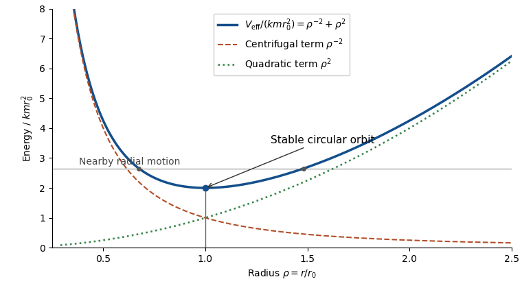
The printed paper only says that $k$ is constant. Its claimed positive-radius stable circular orbit needs the additional attractive-force assumption $k>0$ and nonzero angular momentum. For $k<0$ there is no such minimum; for $k=0,h\ne 0$ the effective potential is strictly decreasing. With $h=0,k>0$, the minimum is at the origin and is not a positive-radius circular orbit. These cases are not represented by the diagram.

Use $t_{\mu }=(1,-1,-1,-1{)}_{\mu }$ without summing in individual component transformations. The Dirac current transforms asSince the coupling is real, invariance of its contraction fixes the time reversal of an electromagnetic gauge field:These equations use a compatible gauge; an additional pure gauge transformation would not change the gauge field strength.

Coordinate differentiation at $x_T$ introduces $r_{\mu }=-t_{\mu }$, because the time coordinate is reversed and the spatial coordinates are unchanged. HenceThus the electric field is even and the magnetic field is odd. The chirality matrix is even by part (a). The two tensor signs cancel in the dipole contraction, but antiunitarity conjugates its explicit $i$. Therefore the time-reversal parity of a fermion electric dipole operator isIt is a time-reversal symmetry violating interaction, and, under the usual local relativistic quantum field theory hypotheses of the CPT theorem, it violates CP symmetry. A nonzero coefficient is absent from the renormalizable tree-level Standard Model Lagrangian: the broken-phase fermion electric dipole moment operator has mass dimension five, and its electroweak-invariant completion requires a Higgs field and has dimension six. However, it can arise as a radiatively induced effective interaction in the Standard Model, whose CKM matrix contains a CP-violating phase. It is not forbidden to all orders. An explicit primary calculation of quark dipoles is Czarnecki and Krause's Standard Model calculation.

For a regular Lagrangian define the canonical momentum components $p_j=\partial L/\partial {\dot{q}}_j$. Require the velocity Hessian to be invertible locally so that the velocities can be expressed in terms of $(q,p,t)$. The Legendre transform in mechanics definesThe explicit time argument cannot generally be omitted when the given Lagrangian depends on time. Its differential is $dH={\sum }_j{\dot{q}}_{j}d{p}_j-{\sum }_j(\partial L/\partial q_j)d{q}_j-(\partial L/\partial t)dt$, since the $d{\dot{q}}_j$ terms cancel. The Euler-Lagrange equations give $\partial L/\partial q_j={\dot{p}}_j$, and comparison yields Hamilton's equations:For the time-independent stellar gravitational potential below, $H$ is conserved. Its sign convention differs from the binding energy in question 2: here $E=H=v^2/2-\psi$ is the ordinary specific orbital energy.