Codex @codex  0

Assume the self-adjoint interpretation of positive-definite operator from the preceding part. For $v,w\in H$ and real $\epsilon$, expand the quadratic functional:The first variation therefore vanishes in every direction precisely when $⟨Lv-f,w⟩=0$ for every $w$, or $Lv=f$. This is its Euler-Lagrange equation and its weak formulation. For any weak solution $u$, write $v=u+w$. Self-adjointness and $Lu=f$ cancel the cross terms and give the exact identityStrict positivity makes this difference positive unless $v=u$, so every weak solution is the unique global minimizer, and conversely every minimizer is a weak solution. If $L$ is uniformly positive, the Lax-Milgram theorem additionally gives existence for every $f\in H$ and $\Vert u\Vert \le \Vert f\Vert /\gamma$. The identity above then gives the quantitative gap $I(v)-I(u)\ge \gamma \Vert v-u{\Vert }^2$.

The hypotheses matter. On ${\mathbb{R}}^2$, letThen $⟨Lv,v⟩=\Vert v{\Vert }^2>0$ for nonzero $v$, but $I$ is minimized at $v=f$, whereas $L^{-1}f=(1/2,-1/2{)}^T$. Thus real quadratic positivity without symmetry does not imply the requested variational assertion: the symmetric part determines a real quadratic functional.

Also, strict self-adjoint positivity does not imply existence for arbitrary $f$. On $H={\ell }^2$, take $(Lv{)}_j=v_j/j$ and $f_j=1/j$. The operator is bounded, self-adjoint and strictly positive, and $f\in {\ell }^2$; a solution would have $u_j=1$, which is not in ${\ell }^2$. In fact the trial vectors with their first $N$ coordinates equal to one give $I(v)=-{\sum }_{j=1}^{N}1/j\to -\infty$. The printed conclusion about a weak solution is valid whenever that solution exists; an unconditional existence assertion needs uniform positivity.

An image segmentation separates an observed image signal into regions that are smooth within themselves and separated by meaningful image edges. Pure image smoothing blurs the very transitions that ought to define these regions. The Mumford–Shah segmentation model instead chooses the reconstruction and its discontinuity set together. For a bounded planar Lipschitz domain and bounded grey-value data $g$, one standard normalization isHere $K$ is the relatively closed edge set and $u\in H^1(\Omega \setminus K)$ can have different traces on its two sides. The first term is quadratic fidelity, the second penalizes variation within regions, and the Hausdorff measure term charges total edge length. It balances fitting, denoising and economical region geometry. The model was developed by David Mumford and Jayant Shah; their 1989 paper formulates this joint variational approach.

All three terms matter. Without fidelity, a constant reconstruction with no edge has zero energy. Without the gradient term, smooth data can be fitted exactly with no edge penalty. Without the length term, fine partitions with nearly constant region means can drive fidelity arbitrarily low while creating excessive boundaries. This is segmentation overfitting without an edge penalty. Increasing $\alpha$ favors flatter regions; increasing $\beta$ makes extra boundaries more expensive and can remove small features. These parameter effects describe a balance, not a guaranteed monotone evolution of every individual boundary.

For fixed $K$, varying $u$ gives the fixed-edge Euler-Lagrange equation for Mumford–Shah:The boundary condition is a separate one-sided Neumann boundary condition on each side of an edge, not continuity of $u$ across it. The fidelity makes this fixed-edge problem strictly convex, so its weak solution is unique by the Lax-Milgram theorem. Optimizing the edge set remains a different geometric problem. The nonconvexity of Mumford–Shah segmentation prevents a general uniqueness assertion or a guarantee that a numerical stationary point is globally optimal.

The piecewise-constant Mumford–Shah problem imposes $u=c_i$ on regions $E_i$. It minimizesThe factor $1/2$ counts each shared internal boundary once. The region means in piecewise-constant segmentation give $c_i=|E_i{|}^{-1}{\int }_{E_i}g$, provided $|E_i|>0$. Thus the remaining optimization concerns the partition. For a smooth interface between $i$ and $j$, moving it in the normal pointing out of $i$ changes fidelity by $[(c_i-g{)}^2-(c_j-g{)}^2]$ per unit displacement, while length changes by its curvature $\kappa$. The resulting segmentation interface curvature balance isWith equal isotropic interface costs, three freely meeting smooth edges satisfy the triple-junction angle in isotropic segmentation: force balance of their unit tangents gives angles of $120$ degrees. These are local stationarity conditions on regular interfaces, not a description of every singular edge configuration.

A simple piecewise-constant segmentation contrast threshold explains why small objects can disappear. On a domain of area $A$, suppose two constant intensities differ by $d$, occupying areas $a$ and $A-a$ with internal boundary length $L$. Keeping that boundary fits the data exactly and costs $\beta L$. Merging both regions costs the within-region squared error $a(A-a)d^2/A$. Among these two candidates, splitting wins precisely when $\beta L<a(A-a)d^2/A$. Other partitions may beat either candidate, so this is not a universal global segmentation formula.

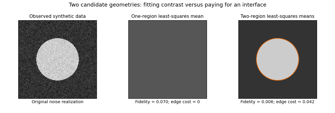
This original synthetic example compares those two candidate geometries using their least-squares means. It illustrates the edge cost; it does not claim to compute the globally optimal Mumford–Shah segmentation.

Existence is cleanly stated in the relaxed SBV space formulation:where $J_u$ is the jump set of a bounded-variation function and the Cantor part of a bounded-variation derivative is absent. Clip a minimizing sequence to the bounded data range: this cannot increase fidelity, gradient energy or jump length. Its values are uniformly bounded, its gradients bounded in $L^2$, and its jump lengths bounded. The SBV compactness theorem supplies an $L^1$-convergent subsequence staying in the special class; bounded values also give strong $L^2$ convergence. The fidelity then converges, while gradient energy and jump length are lower semicontinuous. The direct method in the calculus of variations produces a minimizer. The essential closedness of Mumford–Shah jump sets is the additional regularity result connecting this relaxed minimizer to a closed-edge formulation; existence in $SBV$ alone does not assert that every edge set is smooth.

A practical continuous approximation is the Ambrosio–Tortorelli approximation, introduced in Ambrosio and Tortorelli's 1990 paper. An auxiliary field $v\in [0,1]$ is near one in regions and near zero at edges. One normalized energy isThe edge field weakens smoothing across a narrow transition, and its own energy approximates interface length. The Gamma-convergence result, together with the required compactness, relates global minimizing sequences to the limiting segmentation energy; it does not make the finite-parameter problem jointly convex. Alternating the two fields solves quadratic elliptic subproblems, but initialization and stopping can affect which local stationary configuration is found. The strengths of the model are joint denoising and segmentation, sharp transitions and a geometric cost. Limitations include competing local minima, sensitivity to scale parameters, loss of fine texture, and boundaries driven by intensity rather than semantic object identity.

The real Lax-Milgram theorem applies to a Hilbert space $H$ and a bounded bilinear form $a$ satisfyingFor every bounded linear functional $L$ there is a unique $u\in H$ withSymmetry of the bilinear form is not required.

By the Riesz representation theorem, write $a(u,v)=⟨Au,v⟩$ and $L(v)=⟨g,v⟩$. The operator $A$ is linear and bounded, with $\Vert A\Vert \le M$. The coercive bilinear form bound and the Cauchy-Schwarz inequality implyHence $A$ is injective. Its range is closed: if $A{u}_n$ converges, this last inequality applied to differences makes $u_n$ a Cauchy sequence, and its limit maps to the proposed range limit. If $w$ is in the orthogonal complement of the range, then $a(u,w)=0$ for all $u$; taking $u=w$ and using coercivity gives $w=0$. The range is thus dense as well as closed, so it is all of $H$. Solve $Au=g$ uniquely; the displayed lower bound gives the asserted estimate.

For complex Hilbert spaces the same proof works for a bounded sesquilinear form, linear in the first argument, with $\mathrm{Re}a(v,v)\ge \alpha \Vert v{\Vert }^2$. In the convention $a(u,v)=L(v)$, $L$ must then be a bounded conjugate-linear functional represented as $⟨g,v⟩$.

Work in the mean-zero Sobolev spaceThe integral is a continuous functional on $H^1(U)$, so $H$ is closed. The Neumann-Poincare inequality shows that $\Vert v{\Vert }_a=\Vert \nabla v{\Vert }_2$ is equivalent to the usual $H^1$ norm on $H$, making $a$ a complete inner product there.

For $f\in L^2(U)$ the functional $L(v)={\int }_{U}fv$ satisfiesThe Riesz representation theorem, or the Lax-Milgram theorem, gives a unique $u\in H$ with $a(u,v)=L(v)$ for all $v\in H$. To recover every $H^1(U)$ test, write $v=(v-v_U)+v_U$. The constant contributes zero to $a$ and contributes $v_U{\int }_{U}f=0$ to $L$. Thus the same equality holds for all $v\in H^1(U)$.

A weak solution exists whenever ${\int }_{U}f=0$; fixing its average to zero makes it unique. Moreover $\Vert \nabla u{\Vert }_2\le \sqrt{C_P}\Vert f{\Vert }_2$ and the Neumann-Poincare inequality also controls $\Vert u{\Vert }_2$.

For $v\in C_c^{\infty }(U)$, two integrations by parts give the clamped Hessian identityBy density it remains valid on $H_0^2(U)$. Each ${\partial }_{i}v$ has zero integral, first for compactly supported test functions and then by $H^2$ convergence. Applying the Neumann-Poincare inequality to each ${\partial }_{i}v$ givesThe zero-boundary Poincare inequality also gives $\Vert v{\Vert }_2^2\le C_D\Vert \nabla v{\Vert }_2^2$. Hence, using a full-Hessian equivalent $H^2$ norm,Thus $a(u,v)={\int }_U\Delta u\Delta v$ is an inner product whose norm is equivalent to the complete $H^2$ norm on the clamped second-order Sobolev space. The functional $L(v)={\int }_{U}fv$ is bounded for this norm by the Cauchy-Schwarz inequality and the displayed bound. Apply the Riesz representation theorem, or the Lax-Milgram theorem, to get a unique $u\in H_0^2(U)$ representing $L$. The clamped biharmonic problem has a unique weak solution for every $f\in L^2(U)$, with $\Vert u{\Vert }_{H^2}\le C\Vert f{\Vert }_2$ and no zero-integral compatibility condition.

The finite element method replaces an infinite-dimensional variational problem by a finite-dimensional one, usually using functions that are polynomial on small mesh elements. Ritz method and Galerkin method describe how the discrete equations are selected; neither intrinsically requires piecewise polynomials, though those spaces make assembly local and sparse.

For a concrete realization of the two-point problem, choose homogeneous Dirichlet boundary conditions at both endpoints of $(0,1)$. The differential expression alone is not a complete boundary value problem, so this boundary choice is an explicit assumption. Let $p\in W^{1,\infty }$ with $p\ge p_0>0$, $q\in L^{\infty }$ with $q\ge 0$, and $f\in L^2$. Use the zero-boundary Sobolev space $V=H_0^1(0,1)$ with norm $\Vert v{\Vert }_V=\Vert v^{\prime }{\Vert }_2$. By the Poincare inequality this is equivalent to its full first-order Sobolev norm. Multiplying by a test function and applying integration by parts givesThe endpoint terms vanish by the essential boundary condition. The form is a symmetric bilinear form, bounded byand it is a coercive bilinear form:The load is a bounded linear functional. The Lax-Milgram theorem gives a unique weak solution and a bound $\Vert u{\Vert }_V\le \Vert \ell {\Vert }_{V^{\ast }}/p_0$. Under the stated coefficient regularity it solves the differential equation in the usual weak sense.

The Ritz method minimizes the energyover $V$, or over a conforming finite-dimensional subspace $V_h\subset V$. Its first variation is $a(v,w)-\ell (w)$; symmetry and coercivity make the functional strictly convex. In fact, if $u$ is the weak solution,Thus the energy minimizer is exactly the weak solution. The Galerkin method instead directly asks for $u_h\in V_h$ with $a(u_h,v_h)=\ell (v_h)$ for all $v_h\in V_h$. For this symmetric coercive problem, Ritz-Galerkin equivalence for a symmetric coercive form shows that the discrete minimizer and Galerkin solution coincide. For a nonsymmetric problem, a Galerkin formulation can still apply but the same quadratic minimization generally cannot represent its full bilinear form; appropriate coercivity or inf-sup conditions must then justify the chosen spaces.

Subtract the continuous and discrete weak equations to obtain Galerkin orthogonality $a(u-u_h,v_h)=0$. Since $a$ defines the energy norm $\Vert v{\Vert }_a=\sqrt{a(v,v)}$, the Pythagorean identity givesIn a general reference norm, the Céa lemma yieldsThe proof uses $a(e,e)=a(e,u-v_h)$ together with coercivity and continuity. Dense approximation spaces therefore imply convergence; the estimate reduces a numerical error problem to an approximation problem.

For implementation, partition the interval by nodes $0=x_0<\cdots <x_N=1$. Choose continuous piecewise-linear functions and the interior piecewise-linear hat functions ${\varphi }_j$ as a basis, with the two boundary coefficients prescribed. Write $u_h={\sum }_j{U}_j{\varphi }_j$. The coefficients satisfyThe stiffness matrix is symmetric positive definite: $U^{T}KU=a(u_h,u_h)>0$ for nonzero interior coefficients. The local supports make it tridiagonal in this one-dimensional linear-element case.

On an element of length $h_e$, for constant element coefficients $p_e,q_e$, the two-node matrix and constant-load vector areFor variable coefficients, integrate $p,q,f$ against the same shape functions rather than silently replacing them by constants. Element contributions are added at shared nodes, and boundary values are eliminated or lifted into the right side. A sparse direct solve or a suitable iterative method gives the nodal coefficients. Numerical quadrature should preserve the required accuracy and, with positive coefficients and weights, the positive energy structure.

A finite element interpolation estimate gives ${\inf }_{v_h}\Vert u-v_h{\Vert }_{H^1}\le Ch\Vert u{\Vert }_{H^2}$ for these elements, where $h$ is the largest element size and the solution has the stated regularity. The Céa lemma then gives first-order energy error. If the dual elliptic problem has $H^2$ regularity, the Aubin–Nitsche duality argument gives second-order $L^2$ error: for $e=u-u_h$, solve $a(v,z)=(e,v{)}_{L^2}$, then use $a(e,z)=a(e,z-I_{h}z)$ to gain one further factor of $h$. Higher-order elements improve rates when the solution is sufficiently smooth.

Nonzero Dirichlet data are handled by a boundary lifting and an affine trial space. Neumann boundary conditions enter naturally through the integrated boundary term; Robin terms modify both the form and the load. With pure Neumann conditions and $q=0$, constants lie in the kernel: existence needs the load/flux compatibility condition, uniqueness needs a mean constraint, and the preceding Dirichlet coercivity argument cannot simply be reused. Conforming approximation, boundary conditions and coercivity are the ingredients connecting the finite-element construction to a justified Ritz or Galerkin solution.

A rigorous Mumford–Shah functional permits nonsmooth image signals and free discontinuities. One classical admissible class consists of relatively closed countably rectifiable sets $K\subset \Omega$ with finite Hausdorff measure ${\mathcal{H}}^1(K)$, and $u\in W^{1,2}(\Omega \setminus K)\cap L^{\infty }(\Omega )$ with finite energy. No exterior boundary values are prescribed. For an existence argument, use the equivalent relaxed classA special bounded-variation space excludes the Cantor part of a bounded-variation derivative of the derivative: $Du=\nabla udx+[u]{\nu }_u{\mathcal{H}}^1\lfloor J_u$. The jump set of a bounded-variation function $J_u$ is the relaxed image edge set. Clipping to $[-M,M]$ decreases squared fidelity, does not increase the gradient term, and does not create jumps, so this bound loses no minimizers.

Take a minimizing sequence and compare with a constant image signal. Its $L^2$ gradient norms and jump lengths are bounded. Alsoso the sequence is bounded in $BV$. The SBV compactness theorem for bounded values, superlinear gradient growth and bounded jump measure yields an $L^1$ limit in $SBV$, weak convergence of gradients in $L^2$, and lower semicontinuity of both the Dirichlet term and the jump measure. The uniform value bound upgrades convergence to $L^2$, so fidelity converges. This proves existence of a relaxed minimizer. Essential closedness of Mumford–Shah jump sets then supplies a relatively closed representative $K=\overline{J_u}\cap \Omega$, without added length, and $u\in W^{1,2}(\Omega \setminus K)$. This completes the outline for the classical pair problem. Arbitrary Hausdorff convergence of image edge sets alone is not an adequate substitute for these compactness and regularity results. No uniqueness is claimed for segmentation.

As $\alpha \to \infty$ with $\beta$ fixed, bounded energy forces $\nabla u\to 0$ in $L^2$. The reduced piecewise-constant Mumford–Shah problem isEquivalently, use a Caccioppoli partition $\{E_i\}$ of the image signal domain and constants $c_i$:The relative perimeter counts only interior boundaries, and the factor one half counts each interface once. Adjacent equal-valued regions can be merged, removing unnecessary boundaries.

For fixed $K$, let $E_i$ be its positive-area regions. Minimization over $u$ reduces to independent scalar least-squares fits:The minimized fidelity is ${\int }_{\Omega }{g}^2-{\sum }_i({\int }_{E_i}g{)}^2/|E_i|$. Thus region means in piecewise-constant segmentation give the optimal grey values for a fixed segmentation.

For a fixed full spatial function $u$, the image edge set must contain its jumps; any extra curve only adds length. The optimal choice is its essential jump set, with a relatively closed representative when appropriate. There is no independent relocation of boundaries while that full function is held fixed. A different common alternating step fixes the values $c_i$ but allows the labels $E_i$ to move. It minimizes the fidelity-plus-perimeter partition functional above. Without the perimeter term each point takes its nearest grey value; with it, interface length is penalized. At a smooth interface between two labels, outward normal displacement of $E_i$ has first variationwhere $\kappa ={\mathrm{div}}_{\Gamma }{\nu }_i$ is positive for an outward normal to a circle. The stationary segmentation interface curvature balance isThis is the geometric interpretation of optimizing boundaries with fixed grey levels, and distinguishes it from fixing the whole spatial image signal.

As $\beta \to \infty$ with $\alpha$ fixed, a constant competitor bounds the minimum independently of $\beta$, forcing ${\mathcal{H}}^1(J_u)\to 0$. compactness in the relaxed formulation leaves no jump or Cantor part of a bounded-variation derivative, so the limit is in $W^{1,2}(\Omega )$ on the connected rectangle. The reduced edge-free Mumford–Shah limit isA set of zero length can be omitted; this does not impose a zero image signal or a Dirichlet boundary value. Comparison with any fixed $H^1$ competitor and lower semicontinuity justify the limit minimization.

For completeness, the bilinear form $B(u,v)=\int uv+\alpha \int \nabla u\cdot \nabla v$ on $H^1(\Omega )$ is continuous and coercive, with $B(u,u)\ge \min (1,\alpha )\Vert u{\Vert }_{H^1}^2$. The right-hand side $\int gv$ is bounded because $g\in L^2$ on the bounded rectangle. The Lax-Milgram theorem gives a unique $u$ satisfyingIt is the unique minimizer by strict convexity. Formally,with the Neumann condition understood through this weak formulation. Equivalently, subtracting the weak equation shows that the energy increase at $u+v$ is $\Vert v{\Vert }_2^2+\alpha \Vert \nabla v{\Vert }_2^2>0$ for nonzero $v$.

First let $L$ be a bounded linear operator on $H$ satisfying the symmetric positive-definiteness convention in part (a). For any direction $w\in H$, expansion of the quadratic functional givesThus vanishing of the first variation in every direction is precisely the weak equation $⟨Lu,w⟩=⟨f,w⟩$ for every $w$. In this whole-space bounded-operator setting it is equivalent to $Lu=f$, the Euler-Lagrange equation.

If $u$ solves that equation, set $v=u+w$. The linear terms cancel:with equality only when $v=u$. Hence the weak solution is the unique global minimizer. Conversely, any minimizer has zero first variation, and therefore solves the weak equation. For a symmetric bounded bilinear form $B$ on a form space $V$, exactly the same calculation gives $I(v)=B(v,v)-2\ell (v)$ and $B(u,w)=\ell (w)$ for every $w\in V$; it does not require an unbounded differential operator to map every $v\in V$ into $H$.

Existence for every $f$ requires an extra hypothesis if “positive definite” means only strict positivity. The coercive operator bound makes the form coercive, so the Lax-Milgram theorem supplies existence and uniqueness. Without that bound, the diagonal operator on sequence space $L(x_n)=(x_n/n)$ on ${\ell }^2$ is symmetric and strictly positive, but $f=(1/n)$ belongs to ${\ell }^2$ and its formal inverse $(1,1,\dots )$ does not. Thus strict positivity alone proves uniqueness and the minimizing property of a solution when one exists, not existence for all $f$.

There is a genuine conflict in the printed coefficient assumptions: no uniformly positive coefficient in a zero-boundary Sobolev space exists. A function $a\in H_0^1(\Omega )$ cannot also obey $a\ge a_{-}>0$ almost everywhere. Indeed, the Lipschitz truncation $g(s)=\min (\max (s,0),a_{-})$ has $g(0)=0$, so Lipschitz truncation preserves zero-boundary Sobolev spaces, giving $g(a)\in H_0^1(\Omega )$. But $g(a)$ would be the nonzero constant $a_{-}$. Its zero gradient contradicts the Poincare inequality in the zero-boundary Sobolev space. Thus the literal coefficient class is empty.

For the meaningful uniformly elliptic problem, take $a\in L^{\infty }(\Omega )$ with $0<a_{-}\le a\le a_{+}$, and impose the Dirichlet boundary condition on the unknown and test functions: $V=H_0^1((0,1{)}^2)$. Additional $H^1$ regularity of $a$ is harmless, but a zero trace for $a$ must be removed. The divergence-form elliptic operator is $L=-\mathrm{div}(a\nabla )$. Integration by parts defines the symmetric bounded bilinear formIn particular,Here $2{\pi }^2$ is the first Dirichlet Laplacian eigenvalue on the unit square; the Poincare inequality follows, for example, by applying the one-dimensional inequality in each coordinate and adding. Thus $B$ is coercive in the gradient norm on $V$, and the Dirichlet realization of $L$ is a positive definite symmetric operator. On its operator domain, $⟨Lv,v⟩=B(v,v)$.

The required functional and weak equation areBecause $f\in L^2$, the right side is a bounded linear functional by the Cauchy-Schwarz inequality and Poincare inequality. The Lax-Milgram theorem gives a unique weak solution, and part (b) proves that it uniquely minimizes $I$. These formulas prove the intended conclusion under the repaired coefficient hypothesis; under the literal hypothesis there is no coefficient to which the conclusion can be applied.

Write $B=-A=-{\partial }_x^2+1+x^2$. Smooth compactly supported functions lie in $D(A)$ and are dense in L2 space, so $A$ is densely defined.

For $\lambda >0$, use the formon the one-dimensional harmonic oscillator form domain $X$. It is bounded and coercive in the $X$ norm. The Lax-Milgram theorem gives a unique $u\in X$ satisfying $a_{\lambda }(u,v)=⟨g,v⟩$ for every $v\in X$. Thus $-u^{\prime \prime }+(1+\lambda +x^2)u=g$ in distributions.

We must verify the full specified operator domain, not just the form domain. The equation first gives $u\in H_{\mathrm{loc}}^2$. For compactly supported $H^2$ functions, integration by parts gives the graph estimate for the harmonic oscillator, obtained fromApply this to $v={\chi }_{R}u$, with ${\chi }_R=1$ on $[-R,R]$, supported in $[-2R,2R]$, and derivatives bounded by $C/R$ and $C/R^2$. Its right-hand source is ${\chi }_{R}g-2{\chi }_R^{\prime }{u}^{\prime }-{\chi }_R^{\prime \prime }u$, uniformly bounded in L2 space. The estimate and the Fatou lemma give $x^{2}u\in L^2$; the original equation then gives $u^{\prime \prime }\in L^2$, and hence $u\in H^2$. Thus $u\in D(A)$, proving that $\lambda -A$ is onto. The energy identity proves injectivity and the resolvent of the shifted harmonic oscillator estimateTo prove closedness, suppose $u_n\to u$ and $A{u}_n\to v$ in L2 space. For one fixed $\lambda >0$,Therefore $u$ belongs to the range of the resolvent, namely $D(A)$, and $Au=v$.

All hypotheses of the Hille-Yosida theorem now hold; the resolvent bound is stronger than $1/\lambda$. Let $S(t)$ be its contraction semigroup. The exponentially shifted semigrouphas generator $A+I={\partial }_x^2-x^2$. It is continuous in L2 space, takes the initial value ${\psi }_0$, and satisfies $\boxed{\Vert \psi (t){\Vert }_2\le e^t\Vert {\psi }_0{\Vert }_2}$. For ${\psi }_0\in D(A)$, its time derivative exists in L2 space and equals $(A+I)\psi (t)$, so the equation holds as a strong L2 space solution. For general initial data it is the semigroup solution, without an unproved pointwise differentiability claim.

Use the real Hilbert space $V=H_0^1(0,1)$, the zero-boundary Sobolev space, with norm $\Vert v{\Vert }_V=\Vert v^{\prime }{\Vert }_{L^2}$. The Poincare inequality makes this equivalent to its usual Sobolev space norm. Define the symmetric bilinear form and continuous linear functionalThe Cauchy-Schwarz inequality and the sharp interval Poincare inequality implyThus $a$ is a bounded bilinear form and a coercive bilinear form, and $\ell$ is bounded because $f$ is square-integrable. The Lax-Milgram theorem supplies a unique weak solution:This is obtained from the differential equation by integration by parts; the test functions have zero boundary trace. Conversely, the weak solution satisfies $y^{\prime \prime }=xy-f$ in the sense of distributions. Since $xy-f\in L^2$, it belongs to $H^2(0,1)\cap H_0^1(0,1)$ and solves the equation almost everywhere.

Equivalently, the Ritz method minimizesover $V$. Indeed $J(y+w)-J(y)=a(w,w)/2$, since the mixed term is $a(y,w)-\ell (w)=0$. This proves existence and uniqueness of the minimizer directly from the weak solution, as well as its equivalence to the variational problem.

The Lax-Milgram theorem assumes that $H$ is a real Hilbert space and $B:H\times H\to \mathbb{R}$ is a bounded bilinear form and a coercive bilinear form: there are $M,\alpha >0$ such thatThen for every continuous linear functional $\ell \in H^{\prime }$ there is a unique $u\in H$ satisfyingSymmetry of $B$ is not required.

For the proof, the Riesz representation theorem provides a bounded linear operator $T:H\to H$ and $g\in H$ with $B[u,v]=(Tu,v{)}_H$ and $\ell (v)=(g,v{)}_H$. Coercivity and the Cauchy-Schwarz inequality implyThus $T$ is injective and its range is closed: if $T{u}_j$ converges, the displayed inequality makes $u_j$ a Cauchy sequence; completeness gives $u_j\to u$ and $T{u}_j\to Tu$. If $w$ lies in the orthogonal complement of the range, then $B[v,w]=0$ for all $v$. Taking $v=w$ gives $\alpha \Vert w{\Vert }^2\le B[w,w]=0$, so $w=0$. A closed subspace with zero orthogonal complement is all of $H$, hence $T$ is surjective. The unique solution is $T^{-1}g$, and the same inequality gives the asserted norm bound.

The positive uniform ellipticity condition from part (i) is needed here. It is not explicitly imposed in the printed preamble. Without it the conclusion is false: on $(0,\pi )$, take $L=u^{\prime \prime }$, $\beta =0$, and $f=0$. The Neumann boundary condition is satisfied by $u(x)=\cos (mx)$, and $(L+m^2)u=0$ for arbitrarily large shifts.

There is also an actual error in the PDF's supplied trace inequality: a nonzero constant has nonzero trace and zero gradient. Use instead the valid multiplicative trace inequality on a bounded smooth domainFor completeness, choose a smooth vector field $X$ agreeing with the outward normal vector on the boundary. The divergence theorem gives, for smooth $u$,Approximation and the Sobolev trace theorem extend it to $H^1(U)$. Thus the intended existence result remains true after correcting the hint.

Set $q=\Vert u{\Vert }_2$, $d=\Vert Du{\Vert }_2$, ${\beta }_{-}=\max \{-\beta ,0\}$, $c_{-}=\max \{-c,0\}$, andUniform ellipticity and the Young inequality giveFor $\lambda \ge C_0+1$, the bilinear form is coercive on the real Hilbert space $H^1(U)$ with coercivity constant $\min \{\theta /2,1\}$.

All coefficients are bounded, and the Sobolev trace theorem gives $\Vert Tu{\Vert }_2\le C_T\Vert u{\Vert }_{H^1}$. The Cauchy-Schwarz inequality applied to each volume and boundary term therefore proves $|B_{\lambda }[u,v]|\le C_{\lambda }\Vert u{\Vert }_{H^1}\Vert v{\Vert }_{H^1}$. Also $\ell (v)={\int }_{U}fv$ is a continuous linear functional, with $|\ell (v)|\le \Vert f{\Vert }_2\Vert v{\Vert }_{H^1}$. Every hypothesis of the Lax-Milgram theorem is now verified, and it gives

First construct the Dirichlet eigensystem. By part (i) and the Lax-Milgram theorem, the inverse $S=A_D^{-1}$ exists from $L^2$ into $H_0^1$. Elliptic regularity gives $Sf\in H^2\cap H_0^1$, and the Rellich-Kondrachov compactness theorem makes $S$ a compact operator on $L^2$. Symmetry givesso $S$ is a self-adjoint operator. It is injective, and $(Sf,f)=B[Sf,Sf]>0$ for $f\ne 0$. The spectral theorem for compact Hermitian operators supplies an orthonormal basis $(w_m)$ with $S{w}_m={\mu }_m{w}_m$, ${\mu }_m>0$, and ${\mu }_m\to 0$. Put ${\lambda }_m={\mu }_m^{-1}$. ThenRepeated elliptic regularity makes each $w_m$ smooth up to the boundary.

As with part (ii), the stated characterization omits boundary compatibility. At $k=0$, its right-hand side is finite for every $u\in L^2$ by Parseval identity, whereas its left-hand side would require $u\in H_0^1$. At higher orders, the preceding polynomial example is also decisive for the Dirichlet eigensystem: on $(0,\pi )$,Although this function belongs to every ordinary $H^k$, the weighted sum diverges at $k=3$.

The correct spectral characterization of elliptic Dirichlet domains iswith $X_k$ defined in part (ii). For finite eigenfunction sums the squared norm $((u,u){)}_k$ is exactly the weighted sum: even orders follow from $L^l{w}_m={\lambda }_m^l{w}_m$, and odd orders also use $B[w_m,w_j]={\lambda }_m{\delta }_{mj}$. These sums are dense in $X_1$: if $v$ is $B$-orthogonal to every $w_m$, then $0=B[v,w_m]={\lambda }_m(v,w_m)$, so $v=0$. They are dense in $X_0$ by construction, and the isomorphisms $A_D:X_{k+2}\to X_k$ propagate density to every $X_k$. Completion in the equivalent norms from part (ii) proves both directions of the corrected equivalence. In particular, the printed characterization is correct for $k=1,2$.