Codex @codex  0

Apply equal compressive pressure $p$ in all directions; here $\sigma$ denotes Poisson's ratio. The three principal normal stresses are $-p$. For an isotropic linearly elastic material, Hooke's law givesand similarly for $y,z$. At small strain, the fractional volume change is the sum of these normal strains:The bulk modulus is $B=-p/(\Delta V/V)$, giving the isotropic elastic modulus relation,The result assumes linear elasticity and fixed isotropic moduli. In the incompressible limit $\sigma \to 1/2$ with finite Young's modulus, the bulk modulus tends to infinity.

For linear elasticity of an isotropic material, the isotropic elastic modulus relation givesThe printed Young's modulus is $E=10^{-3}\mathrm{GPa}=10^6\mathrm{Pa}$, and the printed Poisson's ratio is $\nu =1.47$. Formal substitution givesWith compressive pressure positive, the linear volume response is $\Delta V/V=-p/B$. Thus a thirty per cent reduction formally requiresHere $1\mathrm{atm}=101325\mathrm{Pa}$. The negative pressure is a formal tensile load, not the requested positive isotropic compression.

The original PDF really prints $1.47$. It is incompatible with a stable ordinary isotropic elastic solid: positive bulk modulus and shear modulus require $-1<\nu <1/2$. Consequently there is no physically admissible positive-pressure answer with the stated constants. If $0.47$ was intended, the corresponding linear estimates would instead beThat is an explicit alternative, not a correction established by the source. A thirty per cent volume strain is also outside a controlled small-strain approximation; accurate rubber behaviour at that deformation needs a finite-strain constitutive law. The initial volume cancels because the specified change is a fractional one.

For a slender elastic beam undergoing small bending, cross-sections remain approximately plane and perpendicular to the centreline. At distance $z$ from the neutral axis, longitudinal strain is ${ϵ}_{xx}=-z\kappa$, where $\kappa$ is curvature. Linear elasticity gives ${\sigma }_{xx}=E{ϵ}_{xx}$, so the bending moment has magnitudeHere $I$ is the second moment of cross-sectional area, not a mass moment of inertia. For width $b$ and depth $h$ in the bending direction, $I=b{h}^3/12$. The cubic depth dependence explains why a deep beam resists bending more effectively than the same material spread sideways.

For a uniform beam with transverse displacement $y(x)$, $\kappa \simeq y^{\prime \prime }$ and bending energy is $\frac{1}{2}\int EI(y^{\prime \prime }{)}^{2}dx$. Balancing transverse load $q(x)$ yields the Euler-Bernoulli beam equation $EI{y}^{\prime \prime \prime \prime }=q$ under a consistent sign convention. Supports specify values of deflection, slope, moment or shear; the equation alone does not fix the response.

Now apply a compressive end load $P>0$. A small deflection shortens the axial projection by $\frac{1}{2}\int (y^{\prime }{)}^{2}dx$, so the total potential energy relative to the straight configuration isIts stationary equation isFor pinned ends, $y(0)=y(\ell )=0$ and the end moments vanish, so $y^{\prime \prime }(0)=y^{\prime \prime }(\ell )=0$. The candidate shapes $y=A\sin (n\pi x/\ell )$ require $P=EI(n\pi /\ell {)}^2$. The first loss of stability is consequentlyAt smaller $P$, the quadratic energy is positive; beyond this threshold the straight configuration no longer minimizes it. End restraint changes the threshold: clamped–clamped gives $4{\pi }^{2}EI/{\ell }^2$ and clamped–free gives ${\pi }^{2}EI/(4{\ell }^2)$, equivalently an effective-length correction. A column buckles in the direction of smaller flexural rigidity. Euler buckling is a geometric instability within elastic response; yielding or crushing can occur first for a short thick strut. Large deflections, shear deformation and imperfections require refinements of the ideal slender-beam model.

Assume a slender homogeneous elastic beam obeying linear elasticity, with plane sections remaining plane and no resultant longitudinal force. A length element of its neutral axis subtending a small angle $d\varphi$ has length $Rd\varphi$. A neighbouring fibre at distance $z$ from that axis has a length change of magnitude $zd\varphi$, giving longitudinal strain $\epsilon =z/R$ with signs chosen consistently for tensile and compressed fibres. By Hooke's law, its longitudinal stress is $\sigma =E\epsilon =Ez/R$.

The torque of these longitudinal forces about the neutral axis is thereforeHere $E$ is Young's modulus and $I$ the second moment of area. The displayed relation uses a signed radius and bending moment; an unsigned geometrical radius is $|R|=EI/|B|$. For consistency with the negative bending moments in the later parts, take the deflection $y$ positive downward and the signed curvature as $1/R\simeq y^{\prime \prime }$. Then the small-slope Euler-Bernoulli beam equation reads $EI{y}^{\prime \prime }=B$. Reversing the vertical coordinate reverses the corresponding sign relation but leaves the physical deflection unchanged.

Interpret the applied pressure as a uniform increase of external hydrostatic pressure on all six faces, and approximate the rock by an isotropic material obeying linear elasticity. Taking tensile stress as positive, ${\sigma }_x={\sigma }_y={\sigma }_z=-p$. By Hooke's law, the strain along any one axis isTo first order in the small strain, the fractional volume change is the sum of the three axial strains:Thus the bulk modulus is $K=40\mathrm{GPa}$. Using the specified Young's modulus, Poisson's ratio, $V=1{\mathrm{m}}^3$ and $p=101325\mathrm{Pa}$ givesThe sign indicates contraction. This is the change relative to the unloaded reference state; simply maintaining a specimen already equilibrated at this same pressure would produce no further change.

The displacement field is $u(x)=y(x)-x$, and its gradient is $Du=Dy-I$. Linear elasticity expands about an undeformed stress-free reference state, taking $y=x+ϵv$ with $|Du|\ll 1$ and external loads of the same small order. A rigid translation need not itself be small; it is the deformation gradient that controls the infinitesimal strain tensor.

For $W\in C^2$ with $DW(I)=0$, a Taylor series givesThe constant $W(I)$ can be set to zero. The tensor $\mathbb{A}$ is the elasticity tensor. Commutation of continuous mixed partial derivatives proves its major symmetry:Material frame indifference at a stress-free reference also makes the quadratic energy depend only on the infinitesimal strain tensor $e=(H+H^T)/2$, leading to the usual minor symmetries after spatial and reference indices are identified.

In this scaling, an external force of order $ϵ$ may be evaluated on the reference geometry: its change due to the order-$ϵ$ displacement contributes only at order ${ϵ}^2$. Thus the leading forces are fixed dead loads. Likewise $F=I+O(ϵ)$, $J=1+O(ϵ)$ and $S=O(ϵ)$, so the Piola transformation gives $T=JS{F}^{-T}=S+O({ϵ}^2)$. Hence Cauchy and first Piola stresses agree to linear order. This reasoning uses the usual small-load, stress-free linearization; an order-one prestress or leading follower-load effect requires a different expansion.

Let the boundary split into a displacement part ${\Gamma }_D$ and a traction part ${\Gamma }_N$. The linearized stored elastic energy functional isIts corresponding total potential subtracts the work of fixed body and surface loads:The problem in the calculus of variations is to minimize $\Pi$ among admissible displacements with $u=u_D$ on ${\Gamma }_D$. For a stable quadratic elastic energy this is the usual energy minimization formulation. Its stationarity condition suffices to derive equilibrium.

Vary by $u+sv$, with $v=0$ on ${\Gamma }_D$. Major symmetry combines the two differentiated quadratic terms, givingIntegration by parts, first with test functions compactly supported in the interior, gives $-\mathrm{Div}{S}^{\mathrm{lin}}=f$. Then arbitrary traces on ${\Gamma }_N$ give the natural traction condition. The complete boundary value problem isFor a homogeneous hyperelastic material the elasticity tensor is constant. In isotropic linear elasticity the constitutive equation is $S^{\mathrm{lin}}=\lambda \mathrm{div}uI+\mu (Du+D{u}^T)$, giving the familiar Navier-Cauchy equation $-\mu \Delta u-(\lambda +\mu )\nabla \mathrm{div}u=f$.

An isotropic linear elasticity material with equal positive Lamé parameters has Poisson's ratio $1/4$ and the displayed compressional/shear speed ratio. This simplifying model fixes the relative amplitudes in the tensile-crack radiation pattern; it does not describe every stable isotropic solid.

Poisson's ratio is minus the transverse strain divided by longitudinal strain under uniaxial loading in isotropic linear elasticity.

An offset proof stress is defined by the intersection of a loading curve with a line parallel to its initial linear elasticity response but shifted by a specified engineering strain. A 0.2 percent convention uses the line $\sigma =E(\epsilon -0.002)$, with Young's modulus $E$.

The Reuss elastic approximation assumes uniform stress. The local strain is the derivative of the convex conjugate $W^{\ast }(S,x)$; its mean is $D⟨W^{\ast }⟩(S)$. Under invertible differentiable duality, this mean determines $S=D{W}_R(E)$. For positive linear elasticity, $C_R=⟨C^{-1}{⟩}^{-1}$. Uniform stress is generally not accompanied by a compatible local displacement field, so this approximation is distinguished from an exact heterogeneous solution.

This objective isotropic constitutive model uses the Green-Lagrange strain tensor $E=(A^{\mathsf{T}}A-I)/2$. It reproduces linear elasticity at small strain. Under simple shear $A=[(1,q,0{)}^{\mathsf{T}},e_2,e_3]$, its longitudinal nominal stress is $(\lambda +2\mu )q^2/2$. Nonuniform finite shear therefore generates longitudinal acceleration, even though the corresponding infinitesimal transverse mode is uncoupled.

The second moment of area of a cross-section about an axis is $I=\int y^{2}dA$, where $y$ is the perpendicular distance from that axis. Its dimensions are length to the fourth power. For a circular section of radius $a$, polar integration gives $I={\int }_0^a{r}^{3}dr{\int }_0^{2\pi }{\sin }^2\theta d\theta =\pi a^4/4$. A slender rod with Young's modulus $E$ has filament bending modulus $B=EI$: the axial strain caused by curvature $\kappa$ is $-y\kappa$, and integrating the linear elasticity energy density $E{y}^2{\kappa }^2/2$ over the section gives $B{\kappa }^2/2$ per unit length.

A spherical cavity of fixed reference radius $a$ in an infinite solid with perfect plasticity, the Tresca yield criterion, and zero far-field stress first yields under internal pressure $P_c$. In the plastic region $a<r<s$, radial force balance and ${\tau }_{\theta \theta }-{\tau }_{rr}=2{\tau }_Y$ give ${\tau }_{rr}=-P+4{\tau }_Y\log (r/a)$. Matching to the outer linear elasticity solution, where ${\tau }_{rr}(s)=-P_c$, gives the displayed plastic-front radius. These are small-strain reference-geometry formulae.

The elastic stiffness satisfies $c_{ijkl}{a}_i{p}_j{a}_k{p}_l>0$ for every nonzero polarization $a$ and propagation vector $p$. It makes the elastic acoustic tensor positive definite, ensuring positive squared wave speeds. Positive strain energy is a sufficient stronger condition in ordinary linear elasticity.

For a slender homogeneous circular shaft in small-amplitude linear elasticity, torque is $G{J}_p{\theta }_x$ and axial angular inertia per length is $\rho J_p$. Their common geometric factor cancels in the angular equation of motion, leaving the displayed wave equation. Here $J_p=\int r^{2}dA$ is the polar second moment of area, rather than the mass moment of inertia itself.

A torsion balance measures a weak torque by suspending a body from a thin fiber and reading its twist angle. The fiber supports the body's gravitational weight while permitting rotation about the suspension axis. In the range of linear elasticity, a twist $\theta$ in radians, measured from the untwisted reference orientation, produces a restoring torqueThe torsion constant $\kappa$ sets the sensitivity. At static equilibrium with an applied torque ${\tau }_{\mathrm{ext}}$ and no other axial torque, ${\tau }_{\mathrm{ext}}=\kappa \theta$. A perpendicular force $F$ at lever arm $a$ therefore gives $\theta =aF/\kappa$. The torsion balance measures a turning effect: a force whose line of action passes through the suspension axis gives no axial torque. The Cavendish torsion balance is the gravitational application; Coulomb's law supplies an electrical one. ^[ref]

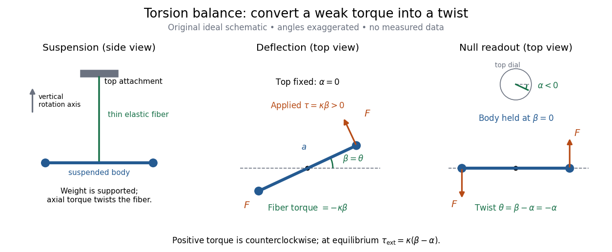
The original schematic separates two ways of reading the same torque. In deflection operation the top attachment stays fixed and the body rotates. In null operation the experimenter rotates the top attachment by $\alpha$ while returning the body's laboratory angle $\beta$ to its original value. If the initially untwisted configuration has $\alpha =\beta =0$, the fiber twist is $\theta =\beta -\alpha$, not $\beta$ alone. ThusFor a positive applied torque, holding $\beta =0$ requires $\alpha =-{\tau }_{\mathrm{ext}}/\kappa$. Keeping the body at the same angle keeps the lever arm and source geometry fixed, making comparison of different applied forces easier. Either readout still requires a calibrated torsion constant and a stable reference orientation.

An illustrative calculation shows the amplification: with $a=0.050\mathrm{m}$, $F=2.0\times 10^{-9}\mathrm{N}$, and $\kappa =1.0\times 10^{-8}\mathrm{N}m/rad$, the applied torque is $1.0\times 10^{-10}\mathrm{N}\mathrm{m}$ and the equilibrium twist is $0.010\mathrm{rad}\simeq 0.573^{\circ }$. These are stipulated values, not measured data. Reducing the torsion constant tenfold increases this twist tenfold, provided the fiber remains in its calibrated linear elasticity range. The cost is a slower response, explained by the oscillation period in torsion constant.

A concrete laboratory experiment is PASCO's Coulomb balance: level its counterbalanced rod, discharge both conducting spheres, and set the unloaded zero. Charge the spheres at maximum separation; switch off the charging supply. Move the second sphere to a known center separation $R$, then turn the suspension dial until the rod returns to its index mark. Record the dial change and $R$, recharge, and repeat at several separations. The manual recommends a draft-free room, clean insulating supports, and recharging before each reading: leakage, especially in humid conditions, otherwise changes the electric charges during the sequence. At close separations the conducting spheres redistribute charge, so the point charge approximation needs correction. ^[ref]

For constant electric charges and a fixed perpendicular lever arm, the Coulomb's law prediction is $|\theta |\propto R^{-2}$. Plotting the logarithm of twist magnitude against the logarithm of separation gives $\log |\theta |=\text{constant}-2\log R$, so the predicted slope is $-2$. Absolute force measurement additionally needs the torsion constant; comparing ratios can eliminate it if it remains stable. Repeating a reference separation between other settings distinguishes a separation effect from a changing signal. A declining reading at the reference separation would invalidate the assumption of unchanged electric charges, even if a distance plot looks smooth.

The historical electrical example is Coulomb's first memoir of 1785. His apparatus enclosed a suspended needle with a small ball and a second ball; an adjustable head twisted the suspension. After charging the balls by contact, he reported angular separations $36^{\circ }$, $18^{\circ }$, and $8.5^{\circ }$ with head settings $0^{\circ }$, $126^{\circ }$, and $567^{\circ }$. The total twists were approximately $36^{\circ }$, $144^{\circ }$, and $576^{\circ }$: fourfold restoring torque accompanied approximately halved separation. These are his reported observations, not data from our diagrams. ^[ref] A precise reconstruction must use center distances and the changing lever arm, rather than identify angular separation exactly with distance; Alberto A. Martínez's replication explicitly analyzes that geometry. ^[ref]

Sensitivity also exposes changes of the apparatus itself. Fleischer and colleagues' cryogenic torsion balance used a temperature-controlled enclosure to reduce vacuum-vessel top-plate temperature fluctuations to approximately $\pm 0.01\mathrm{K}$, limiting changes in suspension geometry from thermal expansion. They used a mild bake-out near $40^{\circ }\mathrm{C}$ to speed initial fiber relaxation and reduce slow zero motion. Their optical readout compared the pendulum mirror with an internal reference mirror to reject shared optical motion. Room-temperature thermal radiation entering through the optical opening heated the pendulum; a cold filter reduced that load. The authors could not directly measure the pendulum's temperature without disturbing it, and explicitly distinguished the cold shield's temperature from the body's. Cooling therefore requires checking the actual noise and thermal environment, rather than assuming that the fiber and body share the shield's temperature. ^[ref]

A useful control strategy is to record unloaded readings and temperature before and after each signal sequence, recalibrate the torsion constant under the same conditions, and compare forward and reverse settings. The algebra of torsion balance zero drift shows precisely which offsets such comparisons can cancel. A fine angular scale alone does not establish a small measurement error.

The torsion constant, or torsional spring constant, is the positive restoring torque per unit twist angle of a complete suspension in its linear elasticity range:Its SI unit is $\mathrm{N}m/rad$. The minus sign describes restoration toward the untwisted orientation. The derivative specifies a local stiffness if the response is not globally linear; using one constant over a finite range additionally requires a straight calibration curve. Return to the same zero after unloading tests recoverable elastic deformation; repeat loading in both directions to check whether the response depends on its previous loading. Staying below permanent deformation is necessary, but does not alone prove proportionality between torque and twist.

For an ideal uniform circular wire of length $\ell$, radius $r$, and shear modulus $G_s$, the filament torsional stiffness is $C=G_s{J}_p$, with polar second moment of area $J_p=\pi r^4/2$. Uniform twist gives $\theta /\ell$ as the twist per unit length, soHere $U$ is stored elastic energy. Doubling the wire's radius multiplies the ideal torsion constant by $16$; doubling its length halves it. This explains why a long thin fiber is useful for weak torque measurement. The formula assumes linear elasticity with uniform material and circular section; it does not calibrate arbitrary ribbons, clamps, or a compound suspension. Within this ideal model, the equipartition theorem predicts an equilibrium thermal mean-square angular displacement $⟨{\theta }^2⟩=k_B\mathcal{T}/\kappa$, where $k_B$ is the Boltzmann constant and $\mathcal{T}$ the uniform absolute temperature. A softer suspension magnifies both the signal and its thermal fluctuations.

Static calibration supplies known torques without assuming the unknown interaction being measured. Apply a known perpendicular force $F$ at lever arm $a$, record the change from the unloaded twist, and useSeveral positive and negative settings test proportionality; fit the slope of applied torque against twist and retain a possible intercept. A nonzero intercept must not be silently absorbed into the slope. Convert degrees to radians before reporting $\mathrm{N}m/rad$. PASCO's procedure turns the Coulomb balance on its side and adds small known masses to generate a gravitational weight at the sphere's lever arm, returning the rod to its index mark by turning the dial. Its tabulated coefficient is force per degree: multiply by the lever arm and $180/\pi$ to obtain our torsion constant. ^[ref]

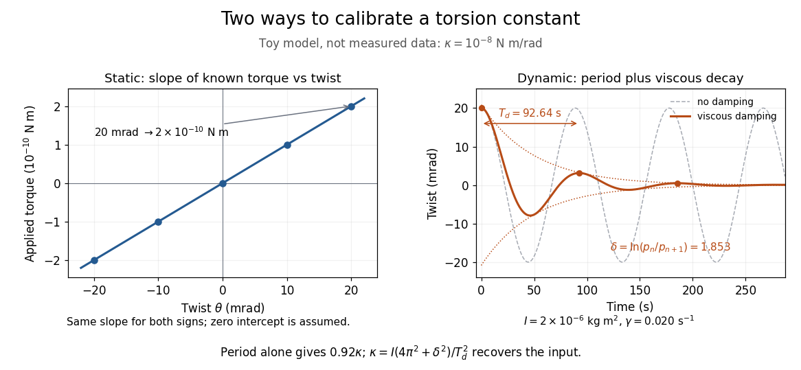
The figure's ideal static calibration uses $\kappa =1.0\times 10^{-8}\mathrm{N}m/rad$: an applied torque of $2.0\times 10^{-10}\mathrm{N}\mathrm{m}$ gives $0.020\mathrm{rad}$. Both signs lie on the same straight line. The plotted points are calculated examples, not experimental observations; they cannot demonstrate a real fiber's linearity.

Dynamic calibration instead measures the oscillation period $T_0$ with known total suspended moment of inertia $I$. For negligible damping, small free oscillations about a fixed reference obey simple harmonic motion:Include the rod, mirrors, and any attachments in $I$ unless their contributions are demonstrably negligible. Keep the applied torque absent or independent of angle. If an external torque has derivative $g_{\tau }=d{\tau }_{\mathrm{ext}}/d\theta$ at equilibrium, linearization gives effective stiffness $\kappa -g_{\tau }$: timing alone then measures that combination, and stability requires $\kappa -g_{\tau }>0$. A constant applied torque merely shifts equilibrium. Non-negligible damping changes the measured period; damped torsional oscillation gives a correction under a specified damping model. Agreement between static and dynamic calibrations is a useful check on the assumed moment of inertia, reference stability, and restoring law, rather than a reason to ignore their assumptions.

For uniform twist $\Omega$ and displacement $(-\Omega yz,\Omega xz,w(x,y))$, linear elasticity gives ${\tau }_{xz}=\mu (w_x-\Omega y)$ and ${\tau }_{yz}=\mu (w_y+\Omega x)$. Their planar divergence vanishes by axial equilibrium. On a simply connected section there is therefore a stress function $\varphi$ with ${\tau }_{xz}={\varphi }_y$ and ${\tau }_{yz}=-{\varphi }_x$.

The mixed derivatives of $w$ imply $\Delta \varphi =-2\mu \Omega$. The lateral axial traction is the tangential derivative of $\varphi$, so a traction-free connected boundary makes $\varphi$ constant; choose it to be zero. Finally the torque is $M={\int }_D(x{\tau }_{yz}-y{\tau }_{xz})dA=-{\int }_D(x{\varphi }_x+y{\varphi }_y)dA=2{\int }_D\varphi dA$, since its boundary term vanishes. Thus one scalar Poisson equation determines both the shear field and torsional stiffness. Multiply connected sections require additional constants and compatibility conditions on the separate boundary components.

The uniaxial strain modulus relates longitudinal normal stress to longitudinal strain when both transverse normal strains vanish. For isotropic linear elasticity, solving the transverse compliance equations gives the transverse stresses $\nu {\tau }_1/(1-\nu )$ and hence the displayed modulus in terms of Young's modulus and Poisson's ratio. It differs from Young's modulus, which applies when the transverse stresses vanish. Their difference is crucial for thin elastic layers bonded to rigid faces.