Codex @codex  0

The mobility correction from a fixed distant sphere givesTaking their ratio and keeping the first nonzero transverse correction yieldsto the stated leading order. Set $b=Y_{\infty }\gg a$. The deflection is $O(a^2/b)$, so replacing $Y$ by $b$ on the right introduces only higher-order errors. Integrating from $X=-\infty$ givesThe maximum occurs at $X=0$, and the deflection and spin in a distant sphere encounter areFor the rotation, use $dt=dX/V$ and $Y=b$ to leading order in the angular velocity from part (b). Its signed angle about the positive $z$ axis isThus the rotation is clockwise when viewed from positive $z$, with the magnitude of the displayed leading term.

The deflection tends back to zero downstream: $Y(+\infty )=Y_{\infty }$. More generally, kinematic reversibility of Stokes flow combined with reflection in the plane $X=0$ makes a passing trajectory fore-aft symmetric. One can see this without using the distant-sphere approximation: the relevant translational hydrodynamic mobility matrix has the form $m_{\perp }(R)I+[m_{\parallel }(R)-m_{\perp }(R)]\mathbf{nn}$. Hence $\dot{X}$ is even in $X$ and $\dot{Y}$ is odd in $X$. Uniqueness of the trajectory through $X=0$ then gives $Y(X)=Y(-X)$.

For $Y_{\infty }=a/100$, the numerical deflection and spin approximations above are invalid: the encounter enters a narrow gap and requires lubrication theory. However, the same return to the incoming offset holds for an ideal passing encounter of perfectly smooth spheres in Stokes flow. Lubrication resistance prevents finite-time contact under a bounded force, and does not itself destroy kinematic reversibility of Stokes flow. Contact, surface roughness or nonhydrodynamic forces could change that conclusion; they are additional physics, not part of the ideal model. This distinction is the fore-aft symmetry of a sedimenting-sphere encounter.

Take $z$ positive upwards and let $f$ denote axial body force per unit volume. With inertia and surface tension omitted, the extensional equations for a slender Newtonian column areMass conservation gives the first equation. The second uses the Trouton ratio three: the leading radial velocity is $u_r=-r{w}_z/2$, the radial normal traction gives $p=p_{\mathrm{ext}}-\mu w_z$, and the axial stress is $-p_{\mathrm{ext}}+3\mu w_z$. An axial control volume balance then gives the displayed equation. The approximation requires a slender column and slowly varying radius.

Let $h=R-a$. Since the container base is closed, the total volume flux at every section is zero. The column carries flux $\pi a^{2}w$, so the annulus carries $-\pi a^{2}w$ and has mean speed of order $a|w|/h$. Its interfacial shear stress is therefore of order $\lambda \mu a|w|/h^2$. Transmitting this stress through the core produces an axial velocity variation of order $\lambda a^2|w|/h^2$. The plug-flow criterion for a column in a low-viscosity annulus is consequently

Use modified pressure $P=p_{\mathrm{ext}}+\rho gz$, removing the annular fluid's hydrostatic pressure. In a local planar gap, with $y=0$ at the column and $y=h$ at the container wall, lubrication theory givesThe required return flux per unit circumference is $q_g=-aw/2$ to leading order in $h/a$. Its pressure-driven component is larger than the Couette component by $a/h$, so the annular return flow around a slumping column givesThe annular shear contribution to the integrated axial force is smaller than this pressure-gradient term by $h/a$. Retaining the leading terms and substituting $f=-(\rho +\Delta \rho )g$ gives the dimensional equationsThe boundary conditions are $w(0,t)=0$ at the base and $w_z(L(t),t)=0$ at the free upper end; the latter expresses zero excess axial extensional stress.

For $\lambda =0$ and initially constant $a=a_0$, put $G=\Delta \rho g/(3\mu )$. Then $w_{zz}=G$, so

For $\lambda >0$, defineThis function records the leading thin-annulus resistance; differences from curvature and the Couette term enter at the already neglected relative order $h/a$. Choose the extensional screening length of a slumping column and the associated scales asHere $h_0=R-a_0$ denotes the initial annular gap in this question. With $Z=z/\hat{z}$, $T=t/\hat{t}$ and $W=w/\hat{w}$, the dimensional equations reduce to

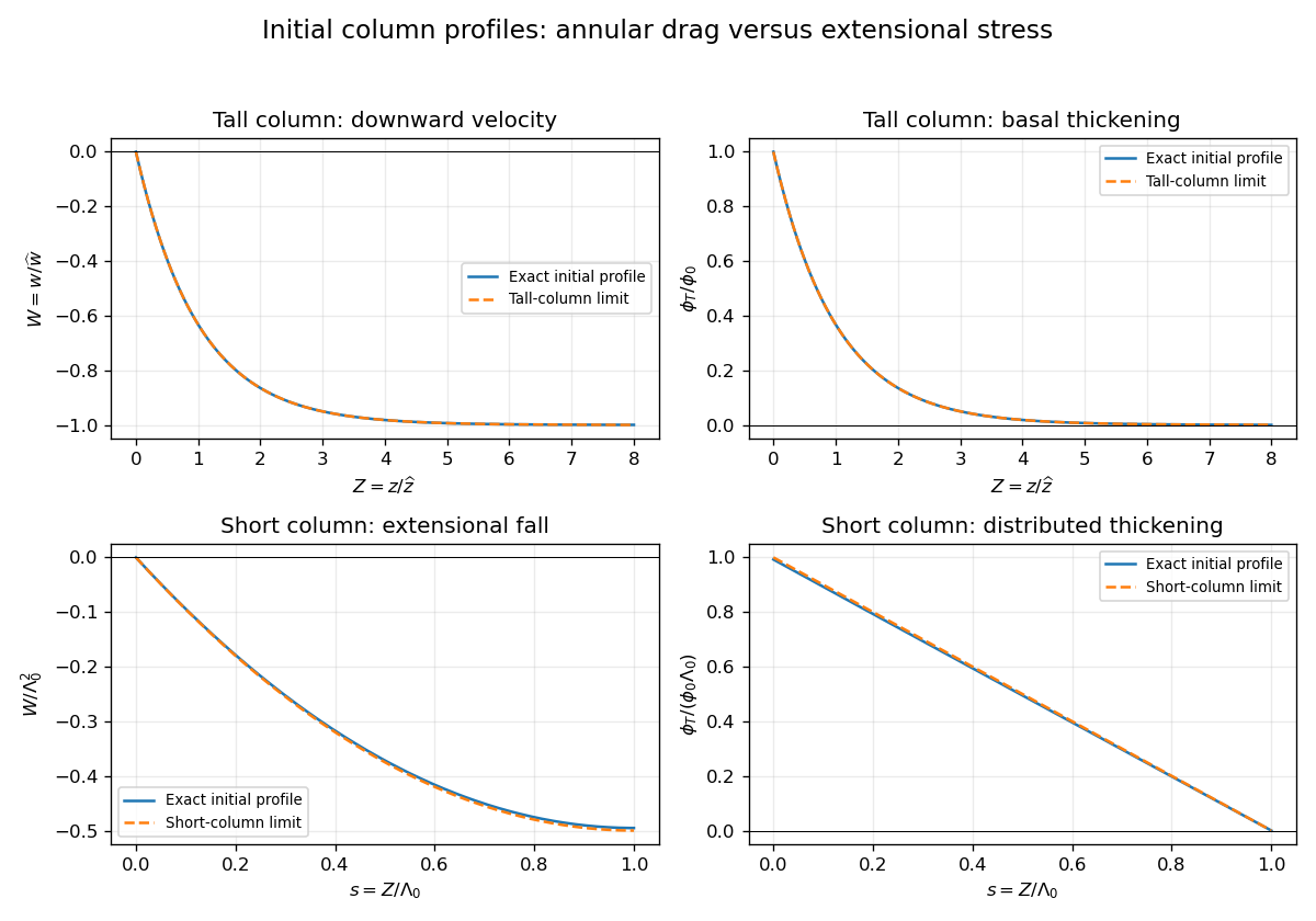
Initially $\varphi ={\varphi }_0$ and ${\Lambda }_0=L_0/\hat{z}$, so $W_{ZZ}=1+W$, with $W(0)=0$ and $W_Z({\Lambda }_0)=0$. The initial velocity profile of an annularly confined column isThe column thickens everywhere below its stress-free top, while that initial thickening rate is zero at the top.

For a tall column, ${\Lambda }_0\gg 1$, the limiting forms away from exponentially small end corrections areThe bulk falls at approximately $-\hat{w}$, where excess weight balances annular hydraulic resistance. Extensional stresses adjust this velocity to zero in a basal boundary layer of thickness $\hat{z}$; almost all thickening occurs there.

For a short column on this scale, ${\Lambda }_0\ll 1$, while still slender, the limits areThe annular-resistance term $W$ is small, so excess weight is balanced predominantly by extensional viscous stress. The top speed is $-\hat{w}{\Lambda }_0^2/2$, recovering the zero-annular-viscosity result. Thus $\hat{z}$ is the vertical distance over which extensional stress communicates the basal constraint before annular resistance screens it. The sketches below use separate natural normalizations for the two limits.

Use pressure with the ambient hydrostatic pressure removed, and let $\Delta P$ be the pressure below the falling sphere minus that above it. Away from the sphere the tube flow is Hagen-Poiseuille flow. The upper and lower clear lengths add to $L$ to leading order in $a/L$, so their pressure drops add:The large exterior reservoir returns this flux with negligible pressure loss compared with the long narrow tube. The sphere is assumed far enough from the ends that entrance effects and its occupied length give only lower-order corrections.

Now use a frame translating downwards with the sphere, and take $z$ positive upwards from its center. The sphere is stationary and the tube wall moves upwards with speed $U$. The narrow gap isIt has axial length scale $a\sqrt{ϵ}$, making lubrication theory appropriate. The sphere-frame flux in a tube is constant: the upward relative flux through the whole section is $\pi a^{2}U-Q$, so its flux per unit circumference isWith $y=0$ on the sphere and $y=h$ on the wall, Couette-Poiseuille flow in a thin gap givesSince $\Delta P=-\int p_{z}dz$, the pressure-jump relation isThe parabolic inner gap can be extended to infinite $z$ because these integrals are dominated by $|z|=O(a\sqrt{ϵ})$. The lubrication resistance integrals for a nearly occluding sphere areSetting $\xi =\tan \theta$ evaluates $J_1=\pi$, $J_2=\pi /2$, $J_3=3\pi /8$, hence

For the force, enclose the fluid between sections just above and below the sphere, including the annular layer. The net upward pressure force is $\pi a^2\Delta P$. The tube wall exerts upward shear traction $\mu u_y(h)$ on this fluid; the sphere exerts a downward force equal to the upward hydrodynamic force $F$ on itself. From the gap solution,The axial control volume force balance therefore gives the control-volume drag formula for a sphere in a tube:Using a control volume avoids having to integrate the curved-sphere normal pressure and tangential shear separately.

With $Q^{\ast }=Q/(\pi a^{2}U)$, $\Delta P^{\ast }=a\Delta P/(6\mu U)$, $q^{\ast }=2q/(aU)$, $F^{\ast }=F/(6\pi \mu aU)$, $I_n^{\ast }=a^{n-1}{I}_n$ and $L^{\ast }=4L/(3a)$, the three flux/pressure equations becomeSolving these linear relations givesThe force relation is $F^{\ast }=\Delta P^{\ast }+\frac{4}{3}{I}_1^{\ast }-q^{\ast }{I}_2^{\ast }$. Substitution first yieldsBecause $I_2^{\ast }/I_3^{\ast }=2ϵ/3$ and $I_1^{\ast }/I_3^{\ast }=2{ϵ}^2/3$, the terms $-2L^{\ast }{I}_2^{\ast }$ and $\frac{4}{3}{L}^{\ast }{I}_1^{\ast }$ are lower order than $L^{\ast }{I}_3^{\ast }$. Keeping the uniformly relevant leading terms givesThe squared $I_2^{\ast }$ is essential; replacing it by $I_2^{\ast }{I}_3^{\ast }$ would give the wrong sign and scaling. This establishes the three drag regimes for a nearly occluding sphere.

For $L^{\ast }\ll {ϵ}^{-1/2}$,The sphere nearly carries the tube's fluid down with it: the far-field flux is close to the piston displacement rate. The relative annular leakage is small in total volume, and the dominant force comes from the local annular shear term. The pressure force associated with the overall tube resistance is smaller.

For ${ϵ}^{-1/2}\ll L^{\ast }\ll {ϵ}^{-5/2}$,The flow remains approximately piston-like, but the dominant force is now the pressure needed to drive Hagen-Poiseuille flow through the long clear tube. Both displayed terms in $q^{\ast }$ are retained because their relative size changes inside this regime without producing an additional leading drag regime.

For $L^{\ast }\gg {ϵ}^{-5/2}$,The large tube resistance makes its net through-flow negligible. The sphere's displaced fluid instead passes upwards relative to it through the thin annular gap, with gap velocity of order $U/ϵ$. Its pressure drop and resulting pressure force dominate.

Finally consider two identical co-moving spheres, with nonoverlapping lubrication regions and the same total clear-tube length to leading order. The common through-flux is not doubled. In the middle regime it is still approximately $\pi a^{2}U$, so the same total tube pressure drop is shared equally between the two identical spheres. The load sharing between co-moving spheres in a tube gives half the single-sphere force on each sphere in regime (ii). In regime (i), drag is set locally by the nearly pressure-balanced annular shear and is unchanged on each sphere. In regime (iii), each sphere must pass essentially its own displacement flux through its annular gap, giving the same local pressure drag as before; adding another pressure jump changes the already small tube flux but not either leading drag. The force is unchanged in regimes (i) and (iii).

The hydrostatic approximation gives $p=\rho g(h-z)$ above the horizontal floor, up to atmospheric pressure. The horizontal Stokes flow equation is $\mu {\mathbf{u}}_{zz}=\rho g\nabla h$, with the no-slip boundary condition at $z=0$ and zero tangential stress on the free surface. Integrating twice gives $\mathbf{u}=(\rho g/\mu )\nabla h(z^2/2-hz)$ and the lubrication gravity-current fluxFor the squeegee lubrication model, use $h_0$ vertically, $\ell =\rho g{h}_0^3/(\mu U)$ horizontally, and $\ell /U$ in time. If $X$ is the laboratory coordinate in the direction of travel, set $x=(X-Ut)/\ell$, $y=Y/\ell$, $t=U{t}_{\mathrm{lab}}/\ell$, and $h=h_{\mathrm{lab}}/h_0$. The blade half-length is $\alpha =L/\ell$. The moving-frame flux is $\mathbf{q}=-h{\mathbf{e}}_x-h^3\nabla h/3$. Conservation of volume gives the dimensionless lubrication equationUsing these scales as representative of the actual flow, lubrication theory requires a small aspect ratio and negligible inertia relative to vertical viscous resistance:The second is the Reynolds number based on $h_0$, multiplied by $h_0/\ell$. Surface tension is neglected as assumed. Large piles, rounded gaps, and narrow end regions need their own local slope and inertia checks if these representative scales cease to describe them.

First supply the introductory scaling and geometry. The leading tangential Stokes equation in a thin gap balances $P/L$ against $\mu U/H^2$. The shear stress scale is $\tau \sim \mu U/H$, so lubrication pressure dominates shear stress:The outer circle, viewed along a ray $r(\cos \theta ,\sin \theta )$ from the inner centre, satisfies $r^2-2\alpha \Delta r\sin \theta +{\alpha }^2{\Delta }^2=(a+\Delta {)}^2$. Expanding its positive root to first order in $\Delta /a$ gives $r=a+\Delta +\alpha \Delta \sin \theta +O({\Delta }^2/a)$, hence $h=\Delta (1+\alpha \sin \theta )$.

Take positive $\Omega$ to mean increasing $\theta$, and put $s=a\theta$, $y=r-a$, $U=\Omega a$. With no-slip boundary conditions at $y=0,h$, lubrication theory givesSteady mass conservation makes $q$ independent of $\theta$. Single-valued pressure requires ${\int }_0^{2\pi }{p}_{\theta }d\theta =0$. Write $I_n={\int }_0^{2\pi }(1+\alpha \sin \theta {)}^{-n}d\theta$ and $D_{\alpha }=1+{\alpha }^2/2$. It follows thatThe tangential fluid tractions on the inner and outer solids, measured in the same increasing-$\theta$ direction, are respectivelyThis sign convention distinguishes the traction on a wall from the corresponding stress component in the fluid.

To leading order the holding force balances the pressure traction on the inner circle. Integration by parts givesUse $p_{\theta }=a{p}_s$ and $\int \sin \theta /(1+\alpha \sin \theta {)}^{n}d\theta =(I_{n-1}-I_n)/\alpha$, with the continuous limit at $\alpha =0$. Substituting the boxed flux yieldsThe zero vertical component also follows from reflection in mathematics in the vertical line: this leaves the geometry and vertical force unchanged, reverses $\Omega$, and Linearity of Stokes flow then requires $F_z=0$.

Pressure gives no moment about either circular wall's own centre. Integrating the viscous shear torque with lever arm $a$ to leading order gives the fluid couplesIndeed $C_i=a^2\int {\tau }_{i}d\theta$ and $C_o=a^2\int {\tau }_{o}d\theta$ at this order. Applied holding or driving couples are the negatives of these fluid couples. They need not cancel because they are moments about different axes. The fluid force on the outer solid equals the holding force $F_x$ on the inner one. Transferring its moment to the inner axis adds $-\alpha \Delta F_x$, so angular momentum balance about a common axis isFor $\alpha =0$ the usual equal and opposite concentric couples are recovered. All these formulas are leading thin-gap expressions at fixed $|\alpha |<1$; taking the contact limit requires maintaining the local slender-gap assumptions.

Work per unit axial length, with $y$ vertically upward and $x$ across the thin gap. In the frame of the downward-translating cylinder, the wall moves upward at speed $U$ and the cylinder surface is stationary. Let $\eta$ be viscosity and use the leading lubrication theoryThe transverse pressure gradient is negligible; solving $\eta u_{xx}=p_y$ with $u(0)=U$, $u(h)=0$ givesThe flux $q$ is constant by incompressibility. Equal ambient pressure at both ends implies $\int p_{y}dy=0$. With $I_j={\int }_{-\infty }^{\infty }{h}^{-j}dy$ and $I_2/I_3=4h_0/3$, this yieldsThe tangential traction on the cylinder isSince $I_2=I_1/(2h_0)$, its integrated force is $-2\eta U{I}_1+4\eta U{h}_0{I}_2=0$. Pressure acts radially on a circular cylinder and contributes no torque; the tangential traction has moment arm $a$ to leading order. HenceFor clarity, the total vertical hydrodynamic force is not zero. Its leading pressure contribution isupward, while the leading shear contribution just calculated vanishes. Thus this model predicts no induced rolling direction: a freely rotating cylinder can remain nonrotating, rather than rolling like a wheel in contact with the wall. This is the torque-free cylinder in a lubrication gap cancellation; finite ends or different boundary conditions would require a different model.

Let $z$ measure distance normal to the plane, with the wall at $z=0$ and the free surface at $z=h$. Take density $\rho$, dynamic viscosity $\mu$, and gravitational acceleration $g$. In lubrication theory, normal momentum balance gives hydrostatic pressure while inertia and streamwise viscous derivatives are smaller. With negligible surface tension and negligible air shear,Apply the no-slip boundary condition $u=v=0$ at $z=0$, and zero leading tangential stress $u_z=v_z=0$ at $z=h$. The velocity profiles areDepth integration gives the volume flux, with $K=\rho g/(3\mu )$:Combining incompressibility with the wall and surface kinematic conditions gives conservation of mass, $h_t+{\partial }_x{q}_x+{\partial }_y{q}_y=0$. Therefore the two-dimensional version of the gravity-driven thin film on an incline satisfiesDirect downslope gravity supplies the advective term, while gradients of the hydrostatic pressure spread the film along the surface. At $\alpha =0$ this reduces to nonlinear gravitational spreading in a horizontal film.

For the horizontal film, part (a) gives the lubrication theory equationThe length scale is fixed at $L$, so balancing $h/t$ against $K{h}^4/L^2$ gives $h\sim (L^2/(Kt){)}^{1/3}$. The draining viscous film on a finite horizontal plate therefore has the long-time similarity solutionAn additive shift of the time origin can represent the initial transient without changing the long-time law. The positive profile is even, with $H^{\prime }(0)=0$ and $H(\pm 1)=0$. Substitution yieldsTo integrate, put $q=H^3{H}^{\prime }$ and use $q^{\prime }=qdq/dH/H^3$. ThenFor $0<\eta <1$ the decreasing branch has $q<0$, so inversion givesThe negative half of the profile follows by symmetry.

At the edge, $\eta (0)=1$. Set $u=(s/H_0{)}^5$ in the integral to obtainHere $B$ is the beta function. Thus $H_0^3=10/(3C^2)$, and the centre thickness is

For $H\ll H_0$, the implicit integral remaining between $0$ and $H$ givesConsequently the edge region of a draining viscous film hasIts slope satisfies $|h_x|\sim (h_0/L)(1-x/L{)}^{-3/4}$ up to a constant factor, so it becomes order one atThe local height is then also $O(\ell )$, violating the shallow geometry required by lubrication theory. A full local flow is needed to turn the fluid over the edge.

The imposed zero thickness is nevertheless a consistent leading outer boundary condition: $\ell /h_0\sim (h_0/L{)}^{1/3}\ll 1$, so the unresolved edge height is small compared with the film's bulk height. It should not be interpreted as an exact pointwise prediction inside the edge region. Moreover, $H^3{H}^{\prime }\to -\sqrt{2/15}{H}_0^{5/2}$ at the right edge, so the outward volume flux remains finite even as the outer thickness tends to zero. The singular slope is what allows this outer solution to describe drainage.

Let $w$ be downward Darcy flux, measured per unit total horizontal area. Neglect the resistance of the displaced phase, capillary pressure, and horizontal subsurface flow. Taking atmospheric pressure as zero, the upper end of the saturated column has pressure $\rho gh$ and its advancing lower end has pressure zero. Across a column of depth $l$, Darcy law therefore givesThe pressure head from the overlying layer supplies $h/l$, and gravity supplies one. Because the new liquid fills a pore volume $\varphi dl$ per unit area, the vertical imbibition under a draining liquid layer obeys $\varphi \dot{l}=w$. Volume conservation gives $h+\varphi l=h_0$, so, until the surface layer is exhausted,The initial condition is understood as a limiting solution of this singular equation. For $0<\varphi <1$, separation of variables givesAt small penetration, expansion of the logarithm yields $t\sim \varphi \nu l^2/(2gk{h}_0)$, henceA sufficient dimensional early-time condition is $t\ll \varphi \nu h_0/(gk)$, for which $l\ll h_0$. The printed $t\ll 1$ needs a chosen time unit or nondimensionalization. In the limiting case $\varphi =1$, $l^2=2gk{h}_{0}t/\nu$ holds exactly until $h=0$. The divergent initial Darcy flux is an idealization of sudden contact with a dry continuum; it cannot describe penetration below the pore scale.

For the spreading surface layer, measure $z$ upwards from the substrate. A thin, slow gravity current has hydrostatic pressure $p=\rho g(h-z)$ and a leading horizontal viscous balance $\nu u_{zz}=g{h}_x$. A no-slip boundary condition at $z=0$ and a stress-free boundary condition at $z=h$ giveThis lubrication gravity-current flux drives horizontal spreading down the surface-pressure gradient. Surface volume conservation is $h_t+q_x=-w$, while conservation in the pores is $\varphi l_t=w$. Combining these balances gives the deep-substrate drainage of a gravity current modelDrainage transfers liquid from the surface layer into the substrate. Indeed $(h+\varphi l{)}_t+q_x=0$.

For definiteness take a one-sided current on $0<x<x_N(t)$, supplied at $x=0$. The imposed volume is per unit span, so $V_0$ has dimensions of area. The boundary conditions and volume conservation constraint areThe source starts from zero injected volume. Initially dry points acquire $l>0$ only when the advancing current reaches them; the formula $h/l$ is not applied outside that region. At the advancing nose these are limiting conditions for a singular drainage equation. For a source feeding two identical sides, each side has half the volume and inlet flux; only the corresponding numerical prefactors change. The integral and inlet-flux conditions are equivalent once the local balance and nose conditions hold.

The physical approximations are lubrication theory, negligible inertia, slowly varying surface height, small pore-scale Reynolds number, and negligible capillary entry pressure. Treating the substrate as vertically draining columns also requires its lateral flow to be negligible and its depth to exceed the penetration depth. The model is valid while surface liquid remains available above each draining column.

For a similarity solution, let $h$ and $l$ scale as $t^a$, and let the current length scale as $t^b$. Since $h/l$ then has no time dependence, drainage requires $a-1=0$. Balancing $h_t$ with the horizontal spreading term gives $a-1=4a-2b$, so $a=1$ and $b=2$. These exponents also give injected volume $t^{a+b}=t^3$, explaining the particular supply law.

Define scaleswhich satisfy $CD=V_0/{\tau }^3$ and $D^2=(g/\nu )C^3$. The cubic-input similarity for a draining gravity current isSubstitution into the two conservation equations giveswhereThus only $K$ and $\varphi$ remain in the dimensionless problem. Its constraints areIntegrating the sum of the two ordinary differential equations verifies that the inlet flux and integral normalization agree. The dimensionless endpoint ${\xi }_N={\xi }_N(K,\varphi )$ is the undetermined multiplicative constant in the length law; solving for it is not required.