Codex @codex  0

Population can move between the levels by electron-impact excitation and de-excitation, spontaneous emission, radiative absorption and stimulated emission. Other collision partners and radiative cascades can matter in a fuller atom. In the elementary coronal approximation, the plasma is dilute, optically thin, steady, and weakly illuminated at the transition frequency. Electron impacts predominantly excite the lower level, while spontaneous emission predominantly empties the upper level; collisional de-excitation and photon trapping are negligible. The population balance isA key condition is $n_e{C}_{21}\ll A_{21}$, together with insignificant external pumping and competing channels. A Maxwellian electron Maxwell-Boltzmann distribution lets the tabulated rate coefficient be expressed using one temperature.

Landau damping is the collisionless decay of a plasma wave through resonant energy exchange with particles whose velocity is close to the wave's phase velocity $v_{\varphi }=\omega /k$. Particles slightly slower than the wave tend to gain energy from it; particles slightly faster can give energy to it. For the decreasing resonant part of a Maxwell-Boltzmann distribution, the net transfer is from the wave to the electrons, so the wave amplitude decays.

In the linear Vlasov equation description this is collisionless phase mixing, not a requirement for frequent particle collisions. Fine-scale structure develops in the velocity dependence of the perturbation even while the macroscopic electric field decreases. The resonant contribution to the growth rate has the sign of $\partial f/\partial v$ at a positive wave phase velocity: a negative slope produces damping, whereas a sufficiently positive slope can drive an instability. A population comparison must be local to the resonance; merely counting all particles faster and slower than the wave is not the criterion.

For the shifted beam Maxwell-Boltzmann distribution,On the rising flank put $u=(V-v)/{\sigma }_b>0$. The positive slope is proportional to $u{e}^{-u^2/2}$, whose derivative is $(1-u^2)e^{-u^2/2}$. Its unique positive maximum is at $u=1$, givingThis is the region where beam drive can most readily overcome the negative plasma slope when that background changes little over the narrow beam width. It is an estimate for the first resonant unstable wave, not a proof that every beam-plasma dispersion relation has its exact marginal phase velocity at this value. Both the total slope and the real dispersion relation determine the exact marginal mode.

For a single-particle state of energy $ϵ$, put $z=e^{\mu /(k_{B}T)}$. The equilibrium mean occupancies areThe Maxwell-Boltzmann distribution is the dilute classical limit. The Fermi-Dirac distribution applies to identical fermions with at most one particle in each complete single-particle state by the Pauli exclusion principle. The Bose-Einstein distribution applies to identical bosons with no such upper occupation bound. The chemical potential fixes total particle number; these are mean state occupancies, not three separately normalized single-particle probability densities. For a number-conserving ideal Bose gas, $\mu$ cannot exceed the lowest single-particle energy.

Take $\mathbf{k}$ to be a wavevector and count periodic-box states with cell volume $(2\pi {)}^3/V$ in momentum space, parameterized by $\mathbf{k}=\mathbf{p}/\hslash$. Write $g_s$ for internal degeneracy. The number of states in a spherical shell is $g_{s}V4\pi k^{2}dk/(2\pi {)}^3$. Since $ϵ=\alpha k$,Thus the one-particle canonical partition function isHere $\beta =1/(k_{B}T)$, $g_s=1$ for one nondegenerate branch, and $g_s=2$ for the spin-half case below. The integral uses ${\int }_0^{\infty }{u}^2{e}^{-u}du=2$. For classical indistinguishable particles, $Z_N=Z_1^N/N!$, givingThe factor three in the energy arises from the linear dispersion relation and three-dimensional state counting; the usual nonrelativistic quadratic-dispersion value $3N{k}_{B}T/2$ does not apply.

For spin-half fermions at $T=0$, all states up to the Fermi energy are occupied. With $g_s=2$,Integrating the occupied energy states givesThese are the corresponding ultrarelativistic ideal Fermi gas formulae with general slope $\alpha$. The nonzero ground-state internal energy and degeneracy pressure reflect the Pauli exclusion principle: particles cannot all occupy the lowest-momentum state. Formally extrapolating the classical equations gives $U,p\to 0$, but Maxwell–Boltzmann statistics is not valid at fixed positive $n$ as $T\to 0$.

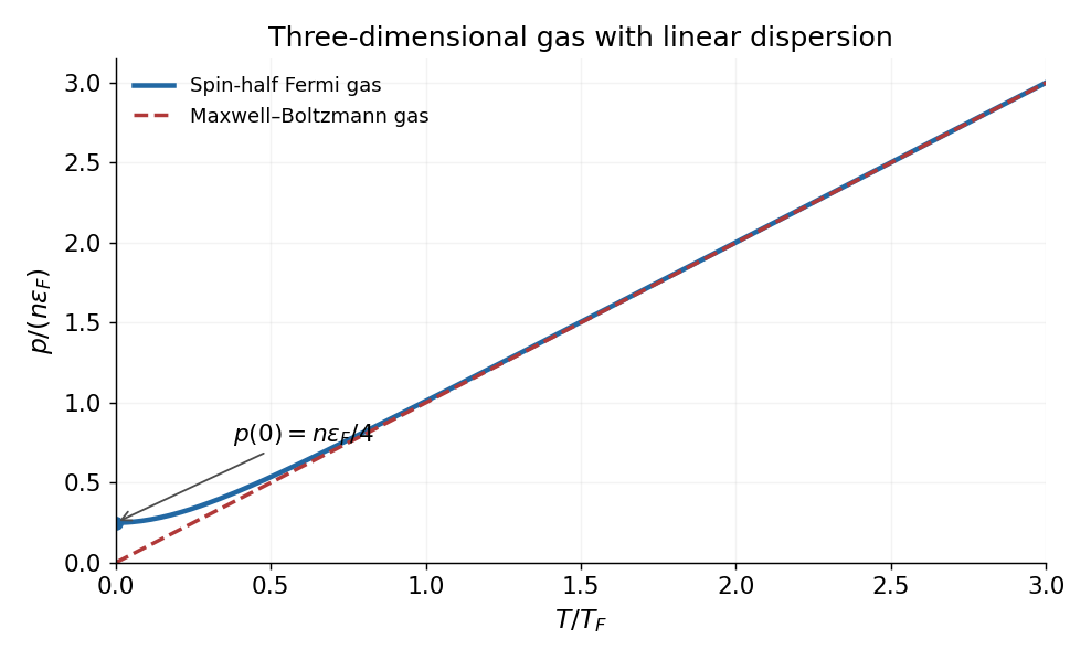
At large $T$, the number equation gives $z\simeq N/Z_1\ll 1$, so expanding the Fermi-Dirac distribution recovers the Maxwell-Boltzmann distribution. A convenient crossover scale is the Fermi temperature,For $T\gg T_F$, both gases have $p\simeq n{k}_{B}T$. At fixed $n$, the Fermi curve begins at $p_0=n{ϵ}_F/4$, has zero initial slope, lies above the classical line, and approaches it at high temperature. For example its low-temperature expansion is $p/(n{ϵ}_F)=1/4+({\pi }^2/6)(T/T_F{)}^2+\cdots$. The plot evaluates the finite-temperature occupation integrals at fixed number density.

If the source's symbol $\mathbf{k}$ is interpreted literally as momentum rather than a wavevector, the state-space cell is $h^3/V$. In that convention replace $\alpha$ in the wavevector-based coefficients and energy scales above by $\hslash \alpha$. The dimensionless thermodynamics and the relation $p=U/(3V)$ are unchanged.

A spatial image after a chosen dark interval is a different readout from continuously recording arrivals at a fixed probe. Here is an original idealised fluorescence imaging model: release a dilute cloud, let it move freely, then apply a short uniform probe pulse. Neglect collisions, residual forces, attenuation and motion during the pulse. Use each image's cloud centre to remove mean drift. Uniform gravity shifts that centre without changing the centred variance.

For each atom let $x(t)=x_0+v_{0}t$ along a horizontal imaging axis. Expanding the square about the expected values gives exactlyNo Gaussian distribution is needed for this variance identity. A jointly Gaussian distribution of initial positions and velocities does make the later density Gaussian. For a separable three-dimensional cloud viewed along $z$, integration along the viewing direction gives the column densityHere $N$ is atom number. Integrating this image along $y$ leaves a one-dimensional Gaussian distribution with standard deviation ${\sigma }_x(t)$. This is a projected density measurement, not a three-dimensional radius or a direct velocity histogram. Under the uniform, optically thin probe assumptions, expected fluorescence is proportional to this column density. A known, independent point spread function with finite variance adds its own variance to the measured width; probe duration and intensity gradients need separate treatment.

For a Maxwell-Boltzmann distribution, $T_x=m{\sigma }_v^2/k_B$, where $m$ is atomic mass and $k_B$ the Boltzmann constant. For a nonthermal distribution this defines a directional second-moment temperature, which need not describe every feature of the distribution. A covariance between position and velocity can initially narrow the cloud even though ${\sigma }_v^2$ is positive. The physical covariance matrix requires $C_{xv}^2\le {\sigma }_{x0}^2{\sigma }_v^2$.

Choose ${\sigma }_{x0}=0.60\mathrm{mm}$, ${\sigma }_v=0.060\mathrm{m}{\mathrm{s}}^{-1}$ and $C_{xv}=-0.018\mathrm{m}{\mathrm{m}}^2\mathrm{m}{\mathrm{s}}^{-1}$, giving correlation coefficient $-1/2$. With $t$ in milliseconds, the numerical variance in square millimetres is $0.36-0.036t+0.0036t^2$. Its minimum occurs at $5\mathrm{ms}$, with standard deviation $\sqrt{0.27}\mathrm{mm}$. These chosen values satisfy the covariance matrix constraint; early contraction is compatible with free motion.

Generate thirteen synthetic variance observations at equally spaced times from $0$ to $30\mathrm{ms}$, adding independent Gaussian noise of standard deviation $0.012\mathrm{m}{\mathrm{m}}^2$. Linear least squares fits all three coefficients in $a+bt+c{t}^2$. The example yields $a\simeq 0.37026\mathrm{m}{\mathrm{m}}^2$, $b\simeq -0.036413\mathrm{m}{\mathrm{m}}^2\mathrm{m}{\mathrm{s}}^{-1}$ and $c\simeq 0.0035820\mathrm{m}{\mathrm{m}}^2\mathrm{m}{\mathrm{s}}^{-2}$. With the chosen approximate sodium mass $m=3.82\times 10^{-26}\mathrm{kg}$, the true $T_x$ is $9.96\mu \mathrm{K}$ and the fitted value is $9.91\mu \mathrm{K}$. This is a fit to generated width data, not historical observations.

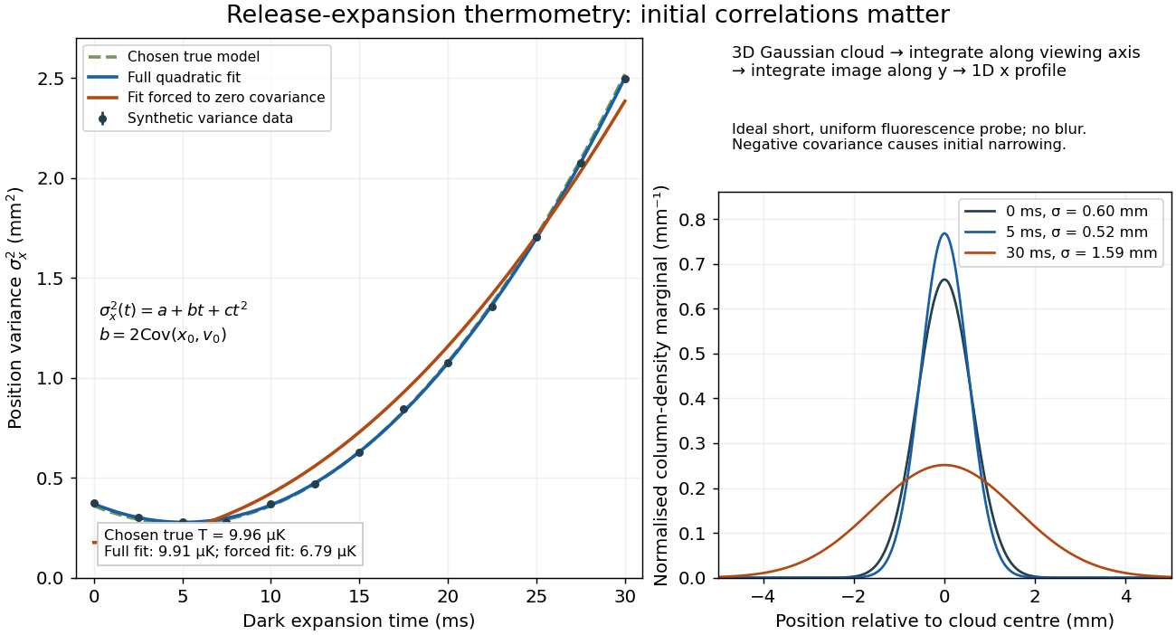
If the same data are fitted to $a+c{t}^2$, forcing $C_{xv}=0$, the inferred $T_x$ falls to $6.79\mu \mathrm{K}$. The omitted term is partly absorbed into both fitted coefficients. In noiseless linear least squares with a free intercept, its precise effect on the quadratic coefficient iswhere the subscript denotes equal-weight moments over the chosen observation times, using one consistent unit system. Since the ratio is positive for distinct nonnegative times, negative $C_{xv}$ biases this estimate downwards. An incorrect release-time origin can also generate a linear term, so fitting it does not by itself identify a physical initial covariance. Timing calibration, spatial resolution, residual magnetic fields and probe-induced recoil energy remain separate controls. Neither a cold-looking image nor a single long expansion time identifies all three coefficients.

The 1988 experiment loaded sodium optical molasses from a slowed atomic beam. After stopping loading, a shutter extinguished the six cooling beams. Released atoms crossed a lower probe; a photomultiplier recorded fluorescence versus arrival time. Calculations integrated the measured initial cloud distribution and an assumed three-dimensional Maxwell-Boltzmann distribution, including gravity and detection geometry. The minimum was $43\pm 20\mu \mathrm{K}$, versus the $240\mu \mathrm{K}$ Doppler cooling limit.^[ref]

Probe separation, probe intensity, cloud density and shutter timing were varied. Fountain-height, horizontal-spreading and release/recapture measurements also gave below-limit results. Geometry remained an uncertainty; agreement among complementary thermometers made a detector artifact less plausible. These measured released atoms, rather than an in-situ velocity distribution.^[ref]

Steven Chu's account connects the explanation to optical pumping, Stark effect shifts and spatially changing electromagnetic polarization; Claude Cohen-Tannoudji's lecture separates this mechanism from subrecoil schemes. Their lectures and William D. Phillips's describe complementary experimental and theoretical routes.^[ref][ref]

If the relative bead velocity $\mathbf{v}$ is independent of its separation and has a centered Maxwell-Boltzmann distribution with $⟨v_i{v}_j⟩=(2k_{B}T/m){\delta }_{ij}$, averaging the drag dissipation of a bead-spring pair gives the displayed gross loss. The cross term vanishes by the zero conditional mean. At zero velocity gradient, this remains $3n\zeta k_{B}T/m>0$, although mechanical stress power is zero. A thermal bath replenishes microscopic kinetic energy at equilibrium. Equating this gross loss to polymer stress power omits heat-bath input and cannot follow from the independently specified Maxwellian velocity distribution. The overdamped free-energy balance of a Hookean dumbbell uses a probability current velocity instead.

A characteristic random particle speed. Here temperature $T_s$ is measured in energy units, and the factor-two convention makes a Maxwell-Boltzmann distribution proportional to $e^{-v^2/v_{\mathrm{th},s}^2}$. Other conventions, such as the one-dimensional standard deviation $\sqrt{T_s/m_s}$, differ by fixed factors.