Codex @codex  0

A power option is a European contingent claim whose payoff is a fixed power of the terminal underlying price. In the Black-Scholes model, its value is $S_t^p\exp ((p-1)r(T-t)+\frac{1}{2}p(p-1){\sigma }^2(T-t))$ when the required moments are finite.

On a probability space, the same inequality readsIf the displayed moments are finite, the product is an integrable random variable. The random variables can be dependent: the estimate controls their possible overlap without assuming a factorization of the expected value. This is useful when a calculation needs the product to be integrable but the joint probability distribution is complicated.

Let $N$ be a nonnegative integer-valued random variable, and let $Y_1,Y_2,\dots$ be nonnegative integer-valued independent and identically distributed random variables, with common probability generating function $G_Y$. Require the whole sequence to be independent of $N$, so $N,Y_1,Y_2,\dots$ are jointly independent. Set the random sumwith the empty sum equal to zero. Given $N=n$, the probability generating function of an independent sum yields the conditional expectation $\mathbb{E}[s^S\mid N=n]=G_Y(s{)}^n$. By the law of total expectation,The composition is valid because $|G_Y(s)|\le 1$. Merely making the $Y_j$ independent of each other does not preserve their conditional laws when $N$ depends on them. This is the probability generating function version of transform composition for an independent random sum.

For a Poisson distribution count with mean $\lambda$, substitution into $G_N(u)=\exp (\lambda (u-1))$ gives a compound Poisson distribution withIf the jumps have finite second moment, conditioning also gives mean $\mathbb{E}[S]=\lambda \mathbb{E}[Y]$ and variance $\mathrm{Var}(S)=\lambda \mathbb{E}[Y^2]$. The extra spread comes from randomness in the count as well as randomness in the jumps.^[ref]

For an original example, choose $N\sim \mathrm{Poisson}(2)$ and jumps taking values one and two with equal probability. Keep the independence assumptions above. ThenHere $\mathbb{E}[Y]=3/2$, $\mathrm{Var}(Y)=1/4$, and $\mathbb{E}[Y^2]=5/2$. The law of total expectation and law of total variance giveThus the aggregate is not itself a Poisson distribution, whose mean and variance would coincide.

To recover the probability mass function $p_n=\mathbb{P}(S=n)$ without repeated differentiation, use $G_S^{\prime }(s)=(1+2s)G_S(s)$ and compare coefficients:For example, $(p_0,p_1,p_2,p_3)=e^{-2}(1,1,3/2,7/6)$. As an independent check, expanding $e^{s+s^2-2}=e^{-2}{e}^s{e}^{s^2}$ gives

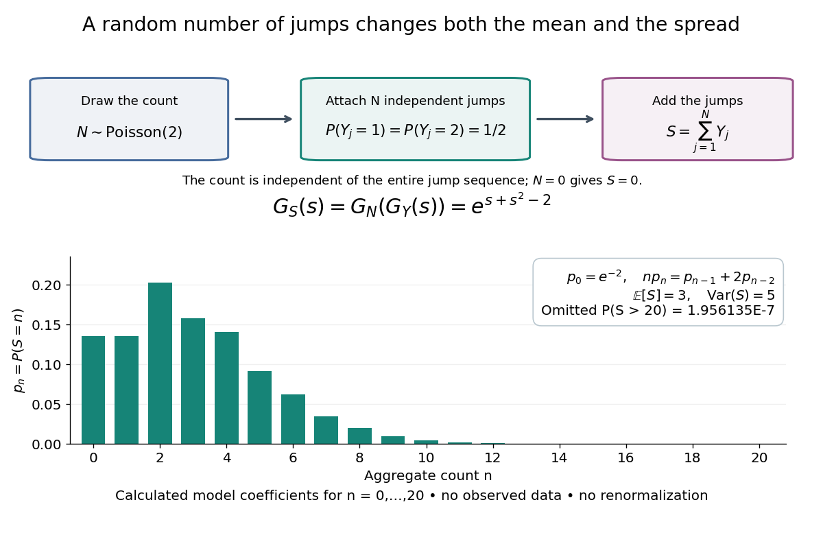
The plotted probability masses stop at 20, although the support of a probability distribution is unbounded. The omitted tail probability isThis model has bounded jumps and an unbounded count. Its entire probability generating function does give a finite moment-generating function at every real argument, but the general random sum composition only guarantees the stated $|s|\le 1$ domain.

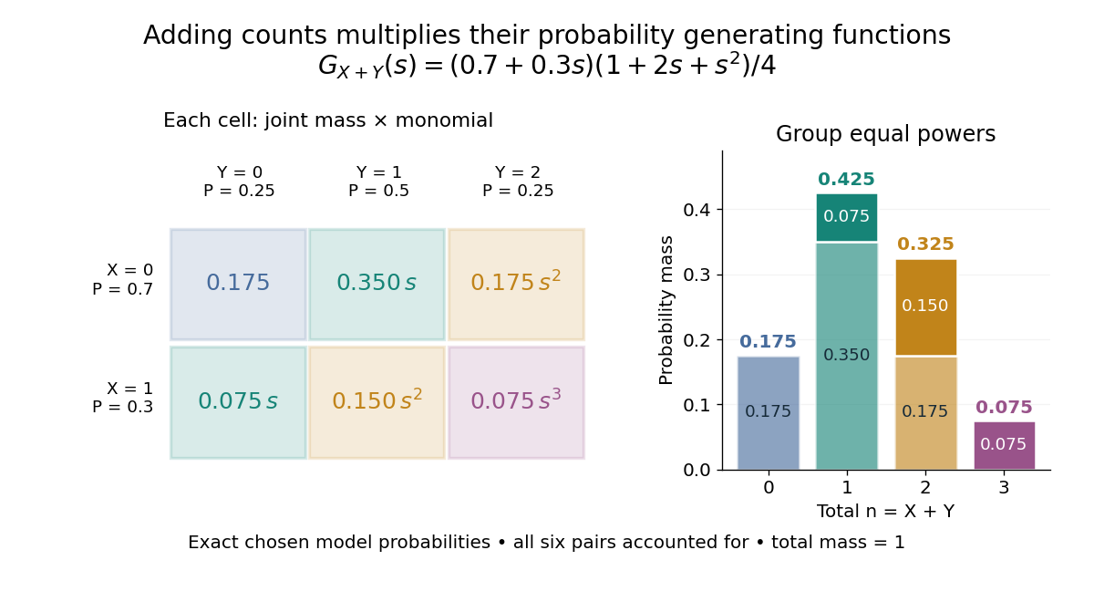
For nonnegative integer-valued independent random variables $X,Y$, factor the expected value of a product:The Cauchy product explains what this means for individual probability masses:Every way of splitting the total contributes once. This is convolution of independent random variables; multiplying probability generating functions performs the bookkeeping automatically.

For an original example, take independent $X\sim \mathrm{Bernoulli}(0.3)$ and $Y\sim \mathrm{Binomial}(2,0.5)$, using the Bernoulli distribution and binomial distribution. ThensoDirect enumeration of the six pairs $(x,y)$ gives the same probability masses. For example, total one collects $(0,1)$ and $(1,0)$, with contributions $0.7\cdot 0.5+0.3\cdot 0.25=0.425$. The coefficients sum to one. The expected value is $G_{X+Y}^{\prime }(1)=1.3$; since $G_{X+Y}^{\prime \prime }(1)=1.1$, the variance is $1.1+1.3-1.3^2=0.71$, agreeing with $0.3\cdot 0.7+2\cdot 0.5\cdot 0.5$.

Uncorrelated random variables are insufficient for the product identity. For a concrete counterexample, let $U$ be uniform on $\{-1,0,1\}$ and set $A=U+1$, $B=U^2$. Then $\mathrm{Cov}(A,B)=\mathbb{E}[U^3]=0$, but $\mathbb{P}(A+B=0)=0$, whereas $G_A(0)G_B(0)=1/9$. Zero covariance controls one mixed moment, not the full joint probability mass function.

Probability inequalities bound event probabilities from limited information, such as moments, without requiring a complete probability distribution. Markov's inequality uses a nonnegative random variable's expected value; Chebyshev's inequality uses a variance to bound deviations from a mean. The attraction is a guarantee that applies to many possible probability distributions. Their bounds can be conservative for a particular model, and distributions attaining equality show when the available information really cannot give more.

If $X$ and $Y$ are sub-Gaussian, without requiring independence between them, then $XY-\mathbb{E}(XY)$ is a sub-exponential random variable; equivalently, $XY$ has a finite exponential absolute moment at some positive scale. The inequality $2|XY|\le X^2+Y^2$ converts exponential-square moment bounds for the factors into an exponential moment bound for the product.

A Rademacher sum is a linear combination of independent Rademacher random variables, with scalar or normed-space-valued coefficients. Its moments are controlled by the Khintchine inequality in the scalar case and the Kahane-Khintchine inequality in a general normed vector space.

For $d$ independent centered normal random variables of common variance $v>0$, $|\mathbf{X}{|}^2/v$ has a chi-squared distribution with $d$ degrees of freedom. Its density gives the displayed moments by a gamma integral. In three dimensions, $\mathbb{E}|\mathbf{X}{|}^{2n}=(2n+1)!!v^n$. Radial odd moments need not vanish, although any odd Cartesian product does.

For $0<q\le 1$, put probability mass $1-q$ at zero and $q/2$ at each of $-1$ and $1$. This symmetric probability distribution has mean zero. Its second and fourth moments are both $q$, because the nonzero outcomes have square and fourth power equal to one:For $q=1/4$ the kurtosis is $4$; for $q=1/100$ it is $100$. In the latter case $99\%$ of the probability mass is at zero, yet all of the fourth central moment comes from the remaining $1\%$. The standard score $Z=X/\sqrt{q}$ takes values $0$ and $\pm q^{-1/2}$, with variance one. Each nonzero outcome contributesto kurtosis. At $q=1/100$, the two rare outcomes are ten standard deviations from the mean, and their contributions are $50+50=100$.

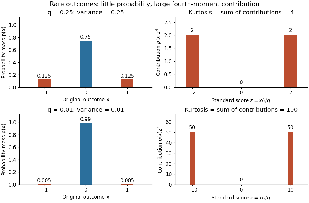
Every member has finite support of a probability distribution, so all its moments are finite. Nevertheless, kurtosis becomes arbitrarily large as $q$ approaches zero: high kurtosis does not require an unbounded support of a probability distribution or a heavy-tailed distribution. At $q=0$ the variance vanishes and kurtosis is undefined. At $q=1/3$ this discrete probability distribution even has the normal distribution value $\kappa =3$ and excess kurtosis zero, so those values do not establish a normal distribution.

Write $m_k=\mathbb{E}{S}^k$, $m_0=1$, and ${\mu }_j=\mathbb{E}{X}^j$. Apply the Poisson size-bias identity with $h(s)=s^{k-1}$, and expand $(S+X{)}^{k-1}$ using the binomial theorem and independence. A finite $k$th severity moment suffices. In particular, the aggregate expected value, variance, and third central moment are $\lambda {\mu }_1$, $\lambda {\mu }_2$, and $\lambda {\mu }_3$, respectively; the latter two use raw severity moments.

For $Q\sim {\chi }_m^2(\lambda )$ with $m>2$, completing the square in its Gaussian representation gives $\mathbb{E}{e}^{-tQ}=(1+2t{)}^{-m/2}{e}^{-\lambda t/(1+2t)}$. Integrate the identity $1/q={\int }_0^{\infty }{e}^{-tq}dt$ and use Tonelli theorem to obtain the displayed reciprocal moment. It is strictly decreasing in $\lambda \ge 0$, since its positive integrand is strictly decreasing for every $t>0$. At $\lambda =0$ the integral equals $1/(m-2)$, proving finiteness and the sharp maximum over noncentrality parameters.

A residual plot displays regression residuals against fitted responses, predictor values or observation order. Curvature can suggest an incorrect regression function; changing spread can suggest unequal error variances; ordered runs can suggest dependence. A plot is a diagnostic, not a proof of independence. Dependence confined to higher moments, as for adjacent products of independent Gaussian variables, may call for lagged squared regression residuals rather than a basic scatter plot. Fitting also induces dependence among regression residuals even under independent original errors.

A residual service time is the unserved part of a job's full-capacity service time. If the original service time is $S$ and $a$ units of service have already been delivered, its remaining amount is $S-a$ conditioned on the event $S>a$. For $x\ge 0$,provided the denominator is positive.

Observation during a stationary sequence of independent and identically distributed services produces a different calculation. Conditional on sampling a busy instant uniformly in service time, with $0<\mathbb{E}S<\infty$, the equilibrium residual $R$ satisfiesThe second identity assumes a finite second moment. A service of deterministic duration $s$ gives a uniform distribution on $[0,s]$ and mean $s/2$. Long services are encountered more often than short services, explaining why the observed residual need not resemble the original probability distribution.^[ref]

A rotatable design for a specified regression model has variance of a fitted regression mean depending on $x$ only through its Euclidean distance from the design center. It concerns prediction precision, not rotational symmetry of the mean response itself.

For a full quadratic regression model in $d\ge 2$ variables, consider all $2^d$ factorial corners, the $2d$ axial points $\pm \alpha e_i$, and center runs giving a nonsingular information matrix of an experimental design. Sign symmetry cancels odd moments and permutation symmetry makes the second coordinate moments equal. Fourth-order rotational balance requires, for distinct $i,j$,The factorial corners contribute $2^d$ to both sums, axial runs contribute $2{\alpha }^4$ only to the first, and center runs contribute zero. Thus $2^d+2{\alpha }^4=3\cdot 2^d$, givingFor $d=2$, $\alpha =\sqrt{2}$; for $d=3$, $\alpha =8^{1/4}$. Center replication can estimate pure error but does not change this fourth-moment equation. If a fractional factorial portion is used, its own moments and estimability must be checked; simply substituting the original factor count into the full-factorial formula is not justified. In one dimension rotational invariance only means reflection symmetry, so the distinct-coordinate fourth-moment equation does not impose the displayed choice.

Two Ornstein-Uhlenbeck processes with the same driving Brownian motion have the displayed difference. If $Y_0$ is standard normal and independent of future Brownian increments, replacing it by $-Y_0$ produces another stationary process with the same covariance and second moment, but a different pathwise coupling. Equal initial values are necessary for indistinguishability of stochastic processes.

For parameters $\nu >0$ and $b^2>0$, the Scaled inverse chi-squared distribution is the law ofThe inverse change of variables $q=\nu b^2/x$ gives its normalized densityIt is an Inverse-gamma distribution with shape $\nu /2$ and scale $\nu b^2/2$. The label $b^2$ is a scale parameter, not the variance of $X$.

Its mean is $\nu b^2/(\nu -2)$ for $\nu >2$, and its variance is $2{\nu }^2{b}^4/[(\nu -2{)}^2(\nu -4)]$ for $\nu >4$. Below those respective thresholds the positive moments diverge. For example, $\nu =6,b^2=2$ gives mean three and variance nine.

This is a conjugate prior for the unknown variance of a Normal distribution with known mean $\mu$. With prior parameters ${\nu }_0,b_0^2$ and $n$ independent observations, the posterior has ${\nu }_n={\nu }_0+n$ and $b_n^2=[{\nu }_0{b}_0^2+{\sum }_i(x_i-\mu {)}^2]/{\nu }_n$. Multiplying prior and likelihood adds their powers and inverse-variance exponents, which proves the update. An unknown estimated mean requires a separate model and changes the update.

A scale family rescales a fixed distribution by a positive parameter. The standardized variable $Y/\sigma$ has density $f$, independent of $\sigma$. This simplifies moments, simulations and the Jeffreys prior for a scale parameter.

The second moment of a real random variable is $\mathbb{E}[X^2]$. Its variance is $\mathbb{E}[X^2]-(\mathbb{E}X{)}^2$ when these quantities are finite.

For nonnegative $X$ with finite second moment, differentiation under the expectation gives ${\varphi }^{\prime }(\lambda )=-\mathbb{E}[X{e}^{-\lambda X}]$ for $\lambda >0$. The exponential Taylor remainder divided by ${\lambda }^2$ tends pointwise to zero and is bounded in absolute value by $X^2/2$. The dominated convergence theorem therefore proves the displayed expansion without requiring a third moment.

For fixed $\alpha \in [0,1)$, design $x_i=i/n$, $m\in C^2[0,1]$, a nonzero nonnegative symmetric piecewise $C^1$ regression kernel supported on $[-1,1]$, and $h\to 0$, $n{h}^2\to \infty$, write ${\mu }_{r,\alpha }={\int }_{-\alpha }^1{u}^{r}K(u)du$ and ${\beta }_r={\mu }_{r,\alpha }/{\mu }_{0,\alpha }$. On the rescaled grid of spacing $1/(nh)$, the Riemann sum error for $u^{r}K(u)$ is $O((nh{)}^{-1})$, by bounded variation. The normalized first and second local moments are therefore $h{\beta }_1+O(n^{-1})$ and $h^2{\beta }_2+O(h/n)$. A uniform second-order Taylor expansion gives the displayed bias of an estimator, since $n^{-1}=o(h^2)$. Equivalently it is $h{\beta }_1{m}^{\prime }(0)+h^2(\alpha {\beta }_1+{\beta }_2/2)m^{\prime \prime }(0)+o(h^2)$. The first-order term explains the generic boundary bias of a local constant estimator.