Codex @codex  0

Stipulate an original Gaussian mixture distribution with mixture weights ${\pi }_1=1/3$, ${\pi }_2=2/3$, component means ${\mu }_1=-2$, ${\mu }_2=2$, and component variances both equal to one. These are chosen statistical parameters, with no observed sample or fitting. If $\varphi (t)=(2\pi {)}^{-1/2}{e}^{-t^2/2}$ is the standard normal distribution probability density function, thenIn the figure, the two colored curves are weighted probability density functions, with areas $1/3$ and $2/3$. Adding their heights at every $x$ gives the black curve. Neither colored curve stops at a dividing line.

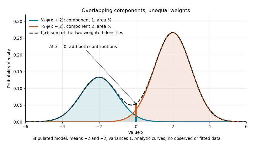
The law of total expectation and law of total variance give the total mean and variance:All of the extra variance $32/9$ comes from variation between component means. Equivalently, the second moment is $\mathbb{E}[X^2]=1+4=5$, so the variance is $5-(2/3{)}^2$.

A mixture distribution is different from a deterministic linear combination of random variables. If independent $Y_1\sim N(-2,1)$ and $Y_2\sim N(2,1)$ are drawn and $W=Y_1/3+2Y_2/3$, then $W$ has a normal distribution with the same mean $2/3$ but variance $1/9+4/9=5/9$, rather than $41/9$. Every draw of $W$ uses both random variables. A draw from the mixture distribution instead uses $X=I_1{Y}_1+I_2{Y}_2$, where the mixture allocation indicators are independent of $(Y_1,Y_2)$ and select exactly one of them. The expression for $f$ adds densities, not simultaneous random outcomes.

Let $X_1,\dots ,X_n$ and $Y_1,\dots ,Y_n$ be two independent samples of independent and identically distributed Hilbert-space-valued random variables, with finite second moments and covariance operators $C_X,C_Y$. To test equality of their expectations, use the pooled covariance operator $C=(C_X+C_Y)/2$. This choice works even when the two population covariance operators differ: under the null hypothesis, the covariance operator of $\sqrt{n/2}(\overline{X}-\overline{Y})$ is exactly $C$.

Let $({\hat{\lambda }}_j,{\hat{\varphi }}_j)$ estimate the eigenvalues and orthonormal eigenvectors of $C$, for example from the average of the two within-sample empirical covariance operators. For fixed $K$, positive retained eigenvalues, a separated retained eigenspace and suitable statistical consistency of these estimates,The proof applies the Hilbert-space central limit theorem to the difference of sample means, then standardizes its first $K$ coordinates and uses Slutsky's theorem. A sufficient simple-eigenvalue condition is ${\lambda }_1>\cdots >{\lambda }_K>{\lambda }_{K+1}$ with ${\lambda }_K>0$.^[ref]

For unequal sample sizes $n,m$, the scaling becomes $nm/(n+m)$ and the relevant population covariance operator is $\{m{C}_X+n{C}_Y\}/(n+m)$. Thus a sample-size-weighted pooled estimate cannot automatically be reused for unequal sizes and unequal covariance operators: its weights must match the variance of the difference being tested.

Here is an explicit joint distribution, for $0<p<0.8$: assign mass $(1+p)e^{-p}-p$ at $(0,0)$, mass $p(1-e^{-p})$ at $(1,0)$, mass $p{e}^{-p}$ at $(1,1)$, and mass $e^{-p}{p}^k/k!$ at $(0,k)$ for $k\ge 2$; all other masses are zero. These are nonnegative: the first is decreasing in $p$, and at $p=0.8$ it is still positive. Summing over rows and columns gives a Bernoulli distribution with mean $p$ and a Poisson distribution with mean $p$, so the joint mass sums to one.

Only $(1,1)$ contributes to the mixed first moment, giving $\mathbb{E}[XY]=p{e}^{-p}$ and the covariance above. The strictly decreasing function $e^{-p}-p$ has a unique zero in $(0,0.8)$, approximately $0.567143$. At that parameter the variables are uncorrelated. They are nevertheless dependent, because $\mathbb{P}(X=1\mid Y=1)=1$ whereas $\mathbb{P}(X=1)=p<1$. The Bernoulli independence from zero covariance result requires both variables to be Bernoulli and does not apply here.

For independent and identically distributed random variables $U_1,\dots ,U_n$ with the continuous uniform distribution on $(0,1)$, the $r$th order statistic has Beta distributionIts probability density function, mean, and variance areThe probability density function is zero outside $[0,1]$; values assigned to its endpoints do not change any probability. Peter Kempthorne's MIT lecture notes derive the uniform order statistic law and these moments. ^[ref].

For $n=5$, the minimum, sample median, and sample maximum correspond to $r=1,3,5$. Their probability density functions are $5(1-t{)}^4$, $30t^2(1-t{)}^2$, and $5t^4$, respectively. The sample median therefore has Beta distribution $\mathrm{Beta}(3,3)$, mean $1/2$, and variance $1/28\approx 0.0357143$. Its cumulative distribution function isFor instance, $\mathbb{P}(U_{(3)}\le 1/4)=53/512\approx 0.103516$. The mean of the minimum is $1/6$, and the mean of the sample maximum is $5/6$. The fixed observed sample median $0.4$ in the order statistic example is one possible outcome; $1/2$ is the average over repeated statistical samples from this uniform distribution.

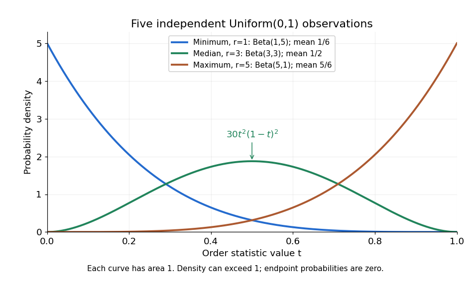
Each curve has area one. The extreme order statistics favor the ends, while the sample median favors the center. The endpoint density height $5$ is legitimate: the probability density function gives area per unit length, rather than point probability. In particular, a continuous uniform distribution has zero probability of producing an endpoint.

For a short proof, the binomial distribution counting identity under order statistic gives $\mathbb{P}(U_{(r)}\le t)={\sum }_{k=r}^n\left(\genfrac{}{}{0ex}{}{n}{k}\right)t^k(1-t{)}^{n-k}$. Taking its derivative cancels consecutive terms, leaving the displayed probability density function. Recognize its normalizing factorial coefficient as that of the Beta distribution, then substitute $\alpha =r$, $\beta =n+1-r$ into the Beta distribution mean and variance formulas. Although the original observations are independent, their order statistics generally are dependent; see the positive covariance of two uniform order statistics.

The Laplace transform of a nonnegative random variable determines its probability law. Indeed, $U=e^{-X}$ takes values in $(0,1]$, and $\mathbb{E}[U^n]={\psi }_X(n)$. Thus the transform determines every moment of $U$; moment determinacy on a compact interval determines the law of $U$, and the injective inverse $X=-\log U$ determines the law of $X$.

For a gyrophase-independent phase-space distribution function, $d^{3}v=2\pi v_{\perp }d{v}_{\perp }d{v}_{\parallel }$. With first adiabatic invariant $\mu =v_{\perp }^2/(2B)$, this gives the measure in the title. When the magnetic field changes, both the measure and any explicit factor $\mu B$ in a moment must be perturbed.

A Markov kernel $P$ has Wasserstein contraction factor $c<1$ for a ground metric $\rho$ whenfor all probability measures for which the distances are finite. Writing $c=e^{-\alpha }$ gives a positive one-step contraction rate $\alpha$. Iteration yields $W_{\rho }(\mu P^n,\nu P^n)\le c^n{W}_{\rho }(\mu ,\nu )$. If $\pi$ is a stationary distribution with finite first moment, this proves geometric convergence in Wasserstein distance to $\pi$ and uniqueness within that moment class. A continuous-time version instead uses factor $e^{-\alpha t}$ for its transition semigroup.

For the random affine recursion $X_{n+1}=a{X}_n+{\xi }_{n+1}$ on the real line with $|a|<1$ and independent finite-first-moment noise, Synchronous coupling uses the same fresh ${\xi }_{n+1}$ for both chains. It gives $|X_{n+1}-Y_{n+1}|=|a||X_n-Y_n|$, hence the contraction factor $|a|$ for $W_1$. The stationary random series ${\sum }_{j\ge 0}{a}^j{\xi }_{-j}$ converges absolutely almost surely because its expected absolute sum is finite. Thus this example also supplies existence, which a uniqueness argument alone would not establish.

The first Wasserstein distance measures the least expected separation achievable when two random variables are coupled with specified marginal probability measures. For a metric space $(E,\rho )$ and measures $\mu ,\nu$ with finite first moments,A transport plan $\pi$ says how much probability mass moves from each starting location to each destination; the distance pays the corresponding metric cost. For point masses on the real line, $W_1({\delta }_a,{\delta }_b)=|a-b|$, because there is only one coupling. In contrast, their Total variation distance is one whenever $a\ne b$. Wasserstein distance therefore records that nearby displacements are small even when the two laws give mass to disjoint sets.

Every coupling gives an upper bound by its expected separation. Conversely, the Kantorovich–Rubinstein theorem gives lower bounds from differences of expectations of Lipschitz functions. The p-Wasserstein distance generalizes the construction by using the $p$th power of the ground metric and then taking a $p$th root.

A sequence of scalar spectral measures ${\mu }_{v,w}^{(n)}$ converges weakly to ${\mu }_{v,w}$ if its integrals against every bounded continuous function converge. A concrete sufficient setting is that all underlying normal-operator spectra lie in one fixed compact set $K\subset \mathbb{C}$ andThe Stone-Weierstrass theorem approximates any continuous function on $K$ uniformly by polynomials in $z,\overline{z}$. Also $\Vert {\mu }_{v,w}^{(n)}{\Vert }_{\mathrm{TV}}\le \Vert v\Vert \Vert w\Vert$: apply Cauchy-Schwarz to the disjoint spectral projections in any finite partition. These uniform total-variation bounds control the approximation errors, so the mixed polynomial tests imply all continuous tests.

On a noncompact real spectrum, a uniform second-moment bound gives uniform tightness for positive scalar spectral measures, but does not alone justify the polynomial approximation step. High-degree polynomial tails require additional uniform integrability, and identifying a limit from all moments needs an additional hypothesis ensuring that these determine the measure. Merely asserting tightness does not supply either missing condition.

For independent and identically distributed random variables with characteristic function $\varphi$, suppose their sample mean converges in Probability to a finite constant $a$. Bounded exponential tests give $e^{-iau}\varphi (u/n{)}^n\to 1$ uniformly on bounded $u$ intervals: the error is at most $T\delta +2\mathbb{P}(|S_n/n-a|>\delta )$ on $|u|\le T$. Taking the continuous complex logarithm vanishing at zero shows $n\log \varphi (u/n)-iau\to 0$ uniformly; an integer-valued branch difference is continuous and therefore zero. For arbitrary $h\to 0$, put $n=\lfloor 1/|h|\rfloor$ and $u=nh$, so $1/2\le |u|\le 1$. Dividing the uniform limit by $u$ proves $\log \varphi (h)/h\to ia$, and thus ${\varphi }^{\prime }(0)=ia$. No absolute first moment is assumed.

Let $X$ have a symmetric probability distribution with $\mathbb{P}(|X|>x)=1/(x\log x)$ for $x\ge e$, mass $1-1/e$ at zero, and no mass with $0<|X|<e$. Then $\mathbb{E}|X|=\infty$, but independent copies satisfy the weak law of large numbers with limit zero. Indeed $n\mathbb{P}(|X|>n)=1/\log n\to 0$. Their symmetric truncations $Y_{n,j}=X_j{1}_{\{|X_j|\le n\}}$ have mean zero and second moment $O(n/\log n)$, so Chebyshev's inequality gives $n^{-1}{\sum }_{j\le n}{Y}_{n,j}\to 0$ in Probability. A union bound shows that the original and truncated sums differ with Probability tending to zero. This also gives a differentiable characteristic function at zero whose derivative cannot be interpreted as an absolutely convergent expectation.

A real degree-$n$ orthogonal polynomial for a positive weight on an interval, with the required finite moments, has exactly $n$ distinct simple zeros in the interval's interior. This places the quadrature nodes of Gaussian quadrature inside its integration domain.^[ref]

To prove it, list the distinct interior roots where the polynomial $p_n$ changes sign, and let $q$ be the product of their linear factors. Then $p_{n}q$ has one constant sign on the interval and is not identically zero. If there were fewer than $n$ sign-changing roots, $q$ would have lower polynomial degree, so orthogonality would give $\int p_{n}qwdx=0$, contradicting positivity of the integral after a choice of sign. There must therefore be $n$ such roots. They exhaust the polynomial degree, proving both simplicity and the absence of additional roots.