Codex @codex  0

Let a nonnegative kernel for density estimation $K$ have integral one, zero first moment and finite second moment ${\mu }_2(K)$. If a probability density function $f$ has bounded second derivative, its kernel density estimator has pointwise bias at most $h^2{\mu }_2(K)\Vert f^{\prime \prime }{\Vert }_{\infty }/2$. Apply the Taylor theorem with Lagrange remainder to $f(x-hu)$ and integrate: the first-order term vanishes and the remainder is bounded by $h^2{u}^2\Vert f^{\prime \prime }{\Vert }_{\infty }/2$. For $K=1_{[-1/2,1/2]}$, ${\mu }_2(K)=1/12$.

A finite nonzero Saffman integral gives $E(k)=L{k}^2/(4{\pi }^2)+o(k^2)$ in the standard isotropic spectrum normalization. This follows by expanding the radial spectral transform at small wavenumber. A further analytic term requires additional correlation moments.

The space-time Probabilists' Hermite polynomial $H_n(x,t)=t^{n/2}{\mathrm{He}}_n(x/\sqrt{t})$ extends polynomially to $t=0$ and solves ${\partial }_t{H}_n+\frac{1}{2}{\partial }_x^2{H}_n=0$. Therefore $H_n(B_t,t)$ is a martingale for a standard Brownian motion, by the Itô formula and Gaussian moments.

A measurable function is square-integrable when the integral of its squared absolute value is finite. Its equivalence class belongs to the L2 space; on a probability space, this means a finite second moment.

A statistical path is a one-dimensional family of probability measures inside a statistical model, passing through a specified baseline $P$. A differentiability in quadratic mean condition gives its score function, the first-order direction of the family in square-root-density coordinates. The path must respect all restrictions of the statistical model, including normalization and any fixed moments.

For independent Steinhaus random variables, condition on their acute angles and use the sharp Rademacher second-moment inequality on the $2d$ sign coefficients $a_i\cos {\theta }_i,i{a}_i\sin {\theta }_i$. Their squared moduli sum to ${\sum }_i|a_i{|}^2$ independently of the angles, so the conditional first moment is at least the same fixed square-root bound. Averaging proves the assertion.

Let $S_n$ be a simple symmetric random walk started at a deterministic value $S_0=s$, and let $T$ be a nonnegative integer-valued stopping time with $\mathbb{E}T<\infty$. The stopped second-moment identity isIn particular, $\mathbb{E}{S}_T^2=\mathbb{E}T$ requires the zero start $s=0$.

For a direct argument, write $S_{T\wedge n}-s={\sum }_{k=1}^n{\xi }_k{1}_{\{T\ge k\}}$. The indicators depend only on the past. Centered independent increments therefore give zero cross terms andFor $m>n$, the same calculation gives the squared L2 norm of the difference as $\mathbb{E}[(T\wedge m)-(T\wedge n)]$, which tends to zero. Thus the stopped positions converge in L2 space, as well as eventually pointwise to $S_T$, and both their first and second moments pass to the limit. This supplies the required justification for an unbounded stopping time; almost-sure convergence alone would not pass the second moment.

Let $X$ have a strictly stable distribution of index $\alpha$, and let $X^{\prime }$ be an independent copy. For integers $1\le k<n$, split a sum of $n$ independent copies into blocks of sizes $k$ and $n-k$. Strict stability of each block and of the full sum givesFor any $0<c<1$, choose rationals $k_m/n_m\to c^{\alpha }$. On the fixed probability space carrying $X,X^{\prime }$, the left side converges almost surely to $cX+(1-c^{\alpha }{)}^{1/\alpha }{X}^{\prime }$. Thus it converges in distribution; since its probability distribution is constant, the limit also has the law of $X$. This proves a self-decomposable distribution with the displayed remainder. The proof does not require any finite moments.

A function into a Banach space is strongly measurable if, outside a null set, it is a pointwise norm limit of measurable simple functions. A measurable function with values in a separable Banach space is strongly measurable: approximate values by a countable collection of balls of shrinking radii and then truncate the resulting countably valued approximants to simple functions. A strongly measurable function is Bochner integral integrable exactly when its norm is integrable. Finite second moments under a probability measure therefore imply existence of its Bochner integral expected value by the Cauchy-Schwarz inequality.

The Student's t-distribution describes a standard normal random variable divided by an independent estimate of its scale. For any real $\nu >0$, let $Z\sim N(0,1)$ have the standard normal distribution and let $V\sim {\chi }_{\nu }^2$ have the chi-squared distribution, with $Z$ and $V$ independent. ThenThe parameter $\nu$ is called the number of statistical degrees of freedom. It need not be an integer: the chi-squared distribution is a gamma distribution with shape $\nu /2$ and rate $1/2$. The independence assumption is essential; specifying only the two marginal distributions does not determine the probability distribution of their ratio.

Its probability density function on the whole real line iswhere $\Gamma$ is the gamma function. Every member is a symmetric distribution about zero. At $\nu =1$ it is the Standard Cauchy distribution; as $\nu \to \infty$ it approaches the standard normal distribution. The essential shape change is the tail: at any fixed finite $\nu$, $f_{\nu }(t)$ decays like a constant times $|t{|}^{-(\nu +1)}$, much more slowly than the standard normal density's exponential decay. Thus it is a heavy-tailed distribution. ^[ref]

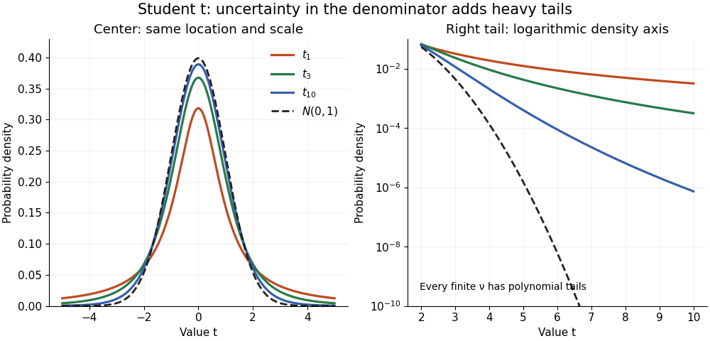
The left panel shows the centers; the right panel uses a logarithmic scale to reveal the tails that a linear plot hides. All four curves have location zero and scale one. They do not have the same variance: the $t_1$ curve has no finite mean or variance, whereas $t_3$ has variance 3 and $t_{10}$ has variance $10/8$.

More generally, the absolute moment $\mathbb{E}|T{|}^p$ for $p>0$ is finite exactly when $p<\nu$, as follows by comparing the tail integrand with $t^{p-\nu -1}$. ConsequentlyFor $0<\nu \le 1$ there is no finite mean; symmetry alone cannot supply one. For $1<\nu \le 2$ the mean exists but the variance is infinite. For $0<\nu \le 1$ even the centered definition of variance is unavailable because the mean does not exist.

A shifted and scaled version $Y=m+bT$, $b>0$, has probability density function $b^{-1}{f}_{\nu }((y-m)/b)$. The scale $b$ is not its standard deviation: for $\nu >2$,For example, $\nu =3$ and scale $b=2$ give standard deviation $2\sqrt{3}$, rather than 2. The distinction matters when using a Student's t-distribution to model data with occasional extreme values, as well as when interpreting a Student t confidence interval.

The tail-sum formula expresses an expected value as the area under a survival function. For every nonnegative random variable $Y$,This Lebesgue integral and the expected value may both be $+\infty$; a probability density function is unnecessary. For a random variable $N$ taking values in the nonnegative integers, the corresponding sum isThe events $\{N>k\}$ and $\{N\ge k+1\}$ coincide because $N$ takes integer values. Thus the strict sum starts at zero, while the inclusive sum starts at one.^[ref]

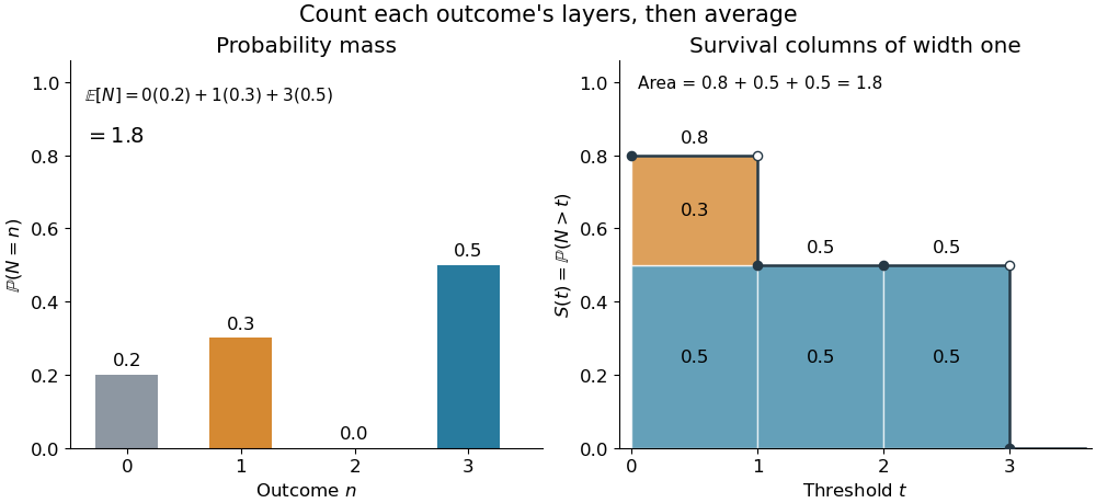
For an original example, let the probability mass function of $N$ beIts expected value computed directly is $0(1/5)+1(3/10)+3(1/2)=9/5=1.8$. The strict tail probabilities at thresholds $0,1,2,3$ are $4/5,1/2,1/2,0$: their sum is again $1.8$. There is no probability mass at two, yet the event $\{N>2\}$ still has probability $1/2$. The survival function has heights $4/5,1/2,1/2$ on the successive intervals $[0,1),[1,2),[2,3)$; each interval has length one, so its integral is the same sum.

The indexing matters numerically. Starting the inclusive sum at zero adds $\mathbb{P}(N\ge 0)=1$, giving $2.8$ for this example. Starting the strict sum at one omits $\mathbb{P}(N>0)=4/5$, giving $1$. For a general nonnegative random variable, replacing $>$ with $\ge$ inside the integral is harmless: the difference is $\mathbb{P}(Y=t)$, nonzero at only a countable set of thresholds. For each positive integer $m$, at most $m$ thresholds can have probability mass at least $1/m$; their countable union contains all thresholds with positive probability mass and has Lebesgue measure zero. This reasoning concerns an integral, not equality of the two survival function conventions at every point.

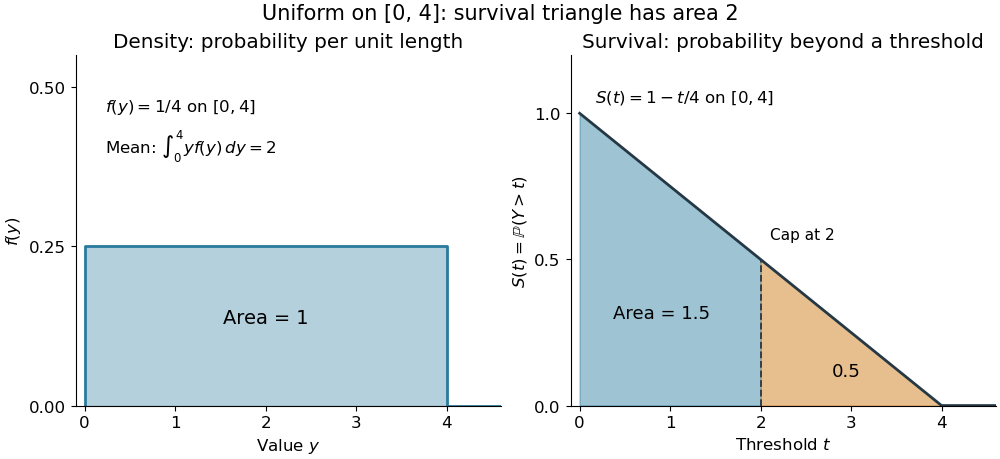
For a continuous original example, take the uniform distribution on the interval $[0,4]$. Its survival function is $S(t)=1-t/4$ for $0\le t\le 4$ and zero for $t>4$. The area is a triangle of base four and height one:Directly integrating against the probability density function gives the same expected value, ${\int }_0^{4}y(1/4)dy=2$. The integral of the probability density function alone is one; it is the survival function whose area is the expected value.

The proof counts layers of each outcome. For a realized value $y\ge 0$, the indicator function $1_{\{y>t\}}$ equals one over an interval of length $y$, soTonelli theorem permits the interchange because the indicator function is nonnegative; no finite expected value is assumed. Similarly, an outcome $N=n$ contributes one indicator random variable for each of the $n$ events $\{N\ge k\}$ that occur:Again Tonelli theorem applies to the nonnegative sum, or equivalently the monotone convergence theorem applies to its partial sums. This exchanges counting layers within each outcome with averaging across outcomes. The existing integer-valued hypothesis in the tail-sum formula explains what changes when the values are not integers; the tail integral formula for moments weights the layers to obtain higher moments.

For an integrable random variable $X$ that can have either sign, apply the nonnegative formula separately to its positive part $X_{+}=\max (X,0)$ and negative part $X_{-}=\max (-X,0)$:Integrability makes both integrals finite. More generally the difference defines an extended expected value when at least one is finite; if both are infinite, subtraction does not define an expected value.^[ref]

Tail probabilities are often easier to measure or bound than a whole probability density function. For a device's survival time, the survival function records the probability of still operating at each threshold; its integral gives the mean operating time. A finite observation window naturally gives the expected value of a capped nonnegative random variable. For a mathematical bound, $\mathbb{P}(Y>t)\le e^{-t/2}$ for all $t\ge 0$ implies $\mathbb{E}[Y]\le {\int }_0^{\infty }{e}^{-t/2}dt=2$. The tail-sum formula turns control of a whole family of events into control of an average.

If $s>0$ and $\Theta$ has the continuous uniform distribution on $(-\pi /2,\pi /2)$, then $Y=s\tan \Theta$ has the Cauchy distribution with location zero and scale $s$. The tangent function is strictly increasing on this interval, so its cumulative distribution function isDifferentiating gives the probability density function $s/[\pi (s^2+y^2)]$. The probability of either endpoint is zero, so including endpoints in the uniform interval does not alter this probability distribution. The slow quadratic decay makes the expected value undefined: its positive and negative parts both have infinite integrals. Its second moment is also infinite, so it has no finite standard deviation.

Fix a common Brownian motion $W$ and a finite horizon $T$. Let positive zero-rate stock prices satisfywith predictable processes $\sigma ,{\sigma }^{\prime }$ bounded in absolute value by a deterministic constant. Their stochastic exponentials are martingales with finite second moments.

If $S_T=a{S}_T^{\prime }$ for a deterministic constant $a$, equality of the expected values forces $a=1$. The martingale identity $S_t=\mathbb{E}[S_T\mid {\mathcal{F}}_t]$ then gives $S_t=S_t^{\prime }$ at each $t$. Continuity of the paths makes this equality hold simultaneously for all times outside a single null set.

Subtract the two Itô integrals. The Itô isometry givesSince $S_t>0$, the coefficients are equal almost everywhere for the product measure $dt\otimes \mathbb{P}$. The common driving Brownian motion is part of the statement.

Perfect positive correlation gives an affine terminal relation that may have a nonzero intercept. It does not supply the proportionality used here; the terminal correlation does not identify adapted stock volatility example demonstrates that distinction.

Suppose a probability density function and its third derivative are bounded. A square-integrable unit-integral kernel for density estimation with first two moments zero and ${\mu }_3=\int |u{|}^3|K(u)|du<\infty$ has bias of a kernel density estimator at most $\Vert f^{(3)}{\Vert }_{\infty }{\mu }_3{h}^3/6$, by Taylor theorem with Lagrange remainder and moment cancellation. independence gives variance at most $\Vert f{\Vert }_{\infty }\Vert K{\Vert }_2^2/(nh)$. The Cauchy-Schwarz inequality bounds the expected centred absolute deviation by the square root of this variance. Adding the bias proves the inequality uniformly in $x$. The choice $h=n^{-1/7}$ gives expected absolute error $O(n^{-3/7})$.

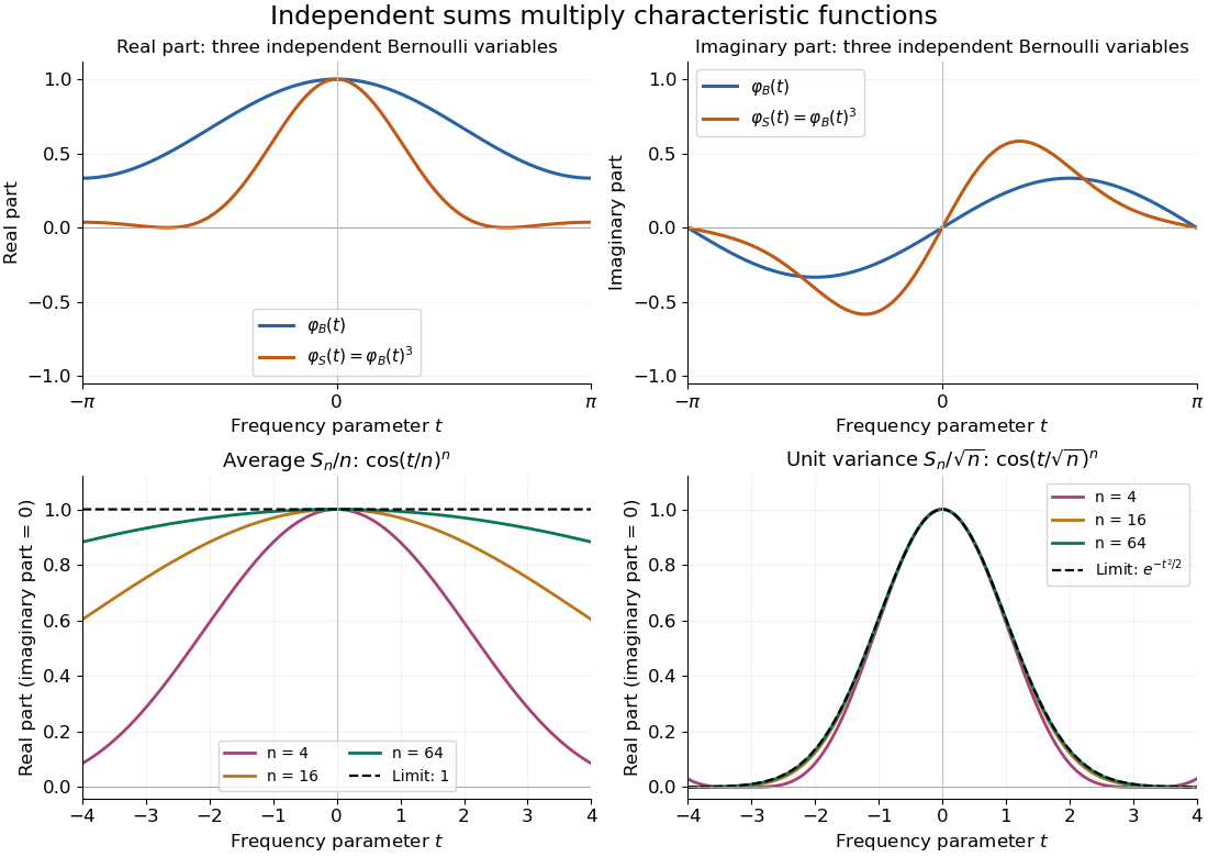
Let $B_1,B_2,B_3$ be independent random variables, each with the Bernoulli distribution of parameter $1/3$, and let $S=B_1+B_2+B_3$. Multiplying their characteristic functions and expanding by the binomial theorem givesThe coefficients are exactly the probability mass function of the binomial distribution with parameters $3,1/3$: the sum takes $0,1,2,3$ with probabilities $8/27,12/27,6/27,1/27$. Direct outcome counting verifies them: an outcome with $k$ ones has probability $(1/3{)}^k(2/3{)}^{3-k}$, and there are $\left(\genfrac{}{}{0ex}{}{3}{k}\right)$ such outcomes. The coefficients sum to one, recovering ${\phi }_S(0)=1$.

At $t=\pi$, ${\phi }_S(\pi )=(1/3{)}^3=1/27$. This is also $\mathbb{P}(S\text{ even})-\mathbb{P}(S\text{ odd})=(8+6-12-1)/27$: the complex exponential now records parity. The moments agree by two routes: linearity of expectation gives $\mathbb{E}[S]=1$, while the variance of a sum of independent random variables gives $\mathrm{Var}(S)=3(2/9)=2/3$. Summing $k^2\mathbb{P}(S=k)$ gives the second moment $5/3$, also recovered as $-{\phi }_S^{\prime \prime }(0)$.

Approximate a compound Poisson distribution of positive claims by a shifted gamma distribution whose first three cumulants agree. Here $m_j=\mathbb{E}{X}^j$ are raw severity moments, while the compound cumulants are $\lambda m_j$. Solve $k+\alpha /\nu =\lambda m_1$, $\alpha /{\nu }^2=\lambda m_2$, and $2\alpha /{\nu }^3=\lambda m_3$ to obtain the displayed parameters. The approximation captures positive skewness, but not the atom $e^{-\lambda }$ at zero. Its shift can be negative; with exponential claims of mean $\mu$ it is $-\lambda \mu /3$. Matching three cumulants alone supplies no general tail-error bound.

A transport-entropy inequality compares the cost of moving one probability measure to another with their relative entropy. For a nonnegative transport cost function $c$ and reference probability measure $\mu$, definewhere $\Pi (\nu ,\mu )$ consists of couplings with those marginals. One common convention is ${\mathcal{T}}_c(\nu ,\mu )\le CD(\nu \Vert \mu )$ for every probability measure $\nu$; the orientation of the relative entropy matters.

For a metric $d$, with the measures having finite first moments, the $T_1(C)$ convention is Wasserstein distance $W_1(\nu ,\mu {)}^2\le 2CD(\nu \Vert \mu )$, while $T_2(C)$ replaces $W_1$ by the second Wasserstein distance $W_2$. The first convention bounds fluctuations of all 1-Lipschitz functions: $\log {\mathbb{E}}_{\mu }{e}^{\lambda (f-{\mathbb{E}}_{\mu }f)}\le C{\lambda }^2/2$. The choice of a squared distance or an unsquared transport cost function is part of the statement, rather than a universal normalization.^[ref]

Let $f_0$ be the triweight kernel and h a twice continuously differentiable density with matching zero mean and variance. Put $e=h-f_0$ and $c=35/32$. Two integrations by parts over its support give $\int e^{\prime \prime }{f}_0^{\prime \prime }=48c[h(1)+h(-1)]+c{\int }_{|x|>1}(360x^2-72)h(x)dx\ge 0$, using the zero mass and second moment of e. Therefore $R(h^{\prime \prime })=R(f_0^{\prime \prime })+R(e^{\prime \prime })+2\int e^{\prime \prime }{f}_0^{\prime \prime }\ge R(f_0^{\prime \prime })$. The endpoint terms matter because the third derivative jumps there.

If $\log S=m+sZ$ with $s>0$, $K>0$ and $Z$ having the standard normal distribution, then for every real $p$,Here $\Phi$ is the standard normal distribution function. Multiplying the normal distribution density by $e^{psZ}$ and completing the square shifts its mean by $ps$ and supplies the factor $e^{p^2{s}^2/2}$; this is a Gaussian exponential tilt. Integrating above or below the shifted threshold proves both formulas. They apply to noninteger and negative powers, including the inverse-price moment $p=-1$. The lower-tail formula gives the European power put formula after a binomial theorem expansion.

A turbulence closure approximates the unclosed higher-order moments in evolution equations for lower-order turbulent statistics. For example, an equation for the velocity correlation tensor involves triple correlations, whose evolution involves fourth-order correlations and pressure. A closure must be checked against conservation laws, realizability and boundary conditions; matching an energy spectrum alone does not establish all these properties.