Codex @codex  0

Differentiating the moment-generating function at zero givesThe second derivative is the second raw moment, so the variance is $M_X^{\prime \prime }(0)-(M_X^{\prime }(0){)}^2$. The assumed exponential integrability justifies these derivatives.

Let $X_f$ have the specified probability density function $f_m$. Splitting the integral into the positive and negative half-lines, and using the Gamma integral ${\int }_0^{\infty }{x}^r{e}^{-sx}dx=r!/s^{r+1}$ for a nonnegative integer $r$ and $s>0$, givesAt $t=2$ or $t=-2$, one term becomes the divergent integral of $x^m$; beyond these endpoints it grows exponentially. Consequently, the full extended-valued moment-generating function isIn particular $M_f(0)=1$, checking normalization of a probability distribution. All absolute moments exist. Direct integration yieldsThe symmetric distribution makes every odd moment zero, so

Now let $X_g$ have probability density function $g_m$. Its moment-generating function would beFor every $t\ne 0$, one summand has exponential growth, which dominates the polynomial decay. HenceThere is no finite moment-generating function on any neighborhood of zero, but some moments still exist. Specifically,ThusFor even $k\ge m+1$, the moment is $+\infty$, so it is not a finite moment. For odd $k\ge m+1$, both the positive and negative contributions have infinite integral, so the expected value is undefined. Cancellation in a Cauchy principal value does not define an expected value. In particular, when $m=0$ there are no finite positive-order moments.

Take a discrete probability distribution on three points:The probabilities are positive and sum to one. Direct calculation givesandNevertheless it is not a symmetric distribution, since $\mathbb{P}(Y=3)=1/10$ while $\mathbb{P}(Y=-3)=0$. Vanishing of just the first and third moments does not force all odd moments to vanish.

Let $X$ have the Pareto distribution with probability density function $f_X(x)=3x^{-4}$ for $x\ge 1$, and zero otherwise. Its normalization of a probability distribution and first two moments follow fromSet $Y=X-3/2$. ThenThe probability distribution of $Y$ is not a symmetric distribution: $Y\ge -1/2$ almost surely, whereas $\mathbb{P}(Y>1/2)=\mathbb{P}(X>2)=1/8>0$ and $\mathbb{P}(Y<-1/2)=0$. For $X\ge 3$ we have $|Y|\ge X/2$, soThus $\boxed{Y=X-3/2}$ has every property required.

First justify that the moments being used exist. For every $r>0$,The bound $|y{|}^k\le k!r^{-k}{e}^{r|y|}$ gives $\mathbb{E}|Y{|}^k<\infty$ for all $k$.

If $Y$ has a symmetric distribution, then $Y$ and $-Y$ have the same probability distribution, so for odd $k$,which forces $\mathbb{E}{Y}^k=0$.

Conversely, suppose every odd moment vanishes. For fixed $t\in \mathbb{R}$, the absolute values of the partial Taylor series for $e^{tY}$ are bounded by $e^{|t||Y|}$, whose expected value is finite by the preceding inequality. The dominated convergence theorem therefore permits termwise expectation:The uniqueness theorem for moment-generating functions implies equality of the probability distributions of $Y$ and $-Y$. Hence

It suffices that the moment-generating function be finite on some open interval containing zero:Equivalently, some two-sided exponential moment exists: $\mathbb{E}{e}^{r|Y|}<\infty$ for some $r>0$. For the forward implication, choose $0<r<\delta$ and use $e^{r|Y|}\le e^{rY}+e^{-rY}$; the converse follows from $e^{tY}\le e^{r|Y|}$ for $|t|\le r$.

Under this weaker hypothesis, all moments exist. For $|t|<r$, dominated convergence justifies the Taylor series argument in (i). Vanishing odd moments gives $M_Y(t)=M_{-Y}(t)$ near zero, and the local uniqueness theorem for moment-generating functions gives the symmetric distribution. The reverse implication follows directly from equality of the two probability distributions.

More generally, it suffices that all moments exist and the probability distribution have moment determinacy: $Y$ and $-Y$ then have identical moments and hence identical probability distributions. Existence of all moments by itself does not provide that uniqueness.

Direct integration of the uniform distribution yields $\mathbb{E}{U}_j=b/2$ and $\mathbb{E}{U}_j^2=b^2/3$. The expectation of a product of independent random variables givesSubtracting the square of the expected value gives the variance:Since $W_n\ge 0$, Markov's inequality implies, for every $\epsilon >0$,Hence $\boxed{W_n\to 0\text{ in probability for }0<b<2.}$ The first moment suffices: the variance need not tend to zero throughout this range.

First take integers $1\le k<n$. For independent copies $X_1,\dots ,X_n$ of $X$, defineThe two blocks involve disjoint families of independent random variables, so $A$ and $B$ are independent. The assumed strictly stable distribution gives $A\stackrel{d}{=}X$, $B\stackrel{d}{=}X$, andTherefore, on any fixed probability space carrying $X$ and an independent copy $X^{\prime }$, their joint probability distribution givesNow fix an arbitrary $0<c<1$ and choose rationals $r_m=k_m/n_m\in (0,1)$ tending to $c^{\alpha }$. Continuity of the real powers gives, on that fixed probability space,The left sides all have the probability distribution of $X$. Since almost sure convergence implies convergence in distribution, their limit has that same probability distribution. HenceThis proves strict stability implies self-decomposability. The limit argument uses no moment-generating function or finite moments, which is essential for general stable distributions.

For $p>1$, the bound $X_k\le 2$ ensures the finite moment $m_p=\mathbb{E}{X}_1^p\le 2^p$. By Jensen's inequality, $m_p\ge (\mathbb{E}{X}_1{)}^p=1$. The process $Z_k=Y_k^p$ is an adapted, nonnegative integrable random variable at each time, and independence givesThus $(Z_k)$ is a submartingale, and $\mathbb{E}{Z}_n=m_p^n$. The Doob maximal inequality for a nonnegative submartingale states that $c\mathbb{P}({\max }_{k\le n}{Z}_k\ge c)\le \mathbb{E}{Z}_n$ for $c>0$. Apply it with $c={\lambda }^p$. Since the power function is increasing on $[0,\infty )$,Combining this with the preceding bound givesThe result is a bound on the running maximum, which is why a maximal inequality for a submartingale, rather than an estimate of the single terminal random variable, is needed.^[ref]

The probabilistic form of Wick's theorem is Isserlis's theorem. If $(Y_1,\dots ,Y_k)$ is a centered random vector with a multivariate Gaussian distribution and covariance matrix $C$, its odd product moments vanish, and, for even $k$,Here ${\mathcal{P}}_2(k)$ is the set of perfect matchings of the $k$ labelled positions. The formula allows repeated coordinates and singular covariance matrices. To see the pairing rule, differentiate the moment-generating function $\exp (t^{T}Ct/2)$ once in each coordinate and set $t=0$: only terms pairing all differentiated coordinates survive, each with the displayed product of covariances.

Take $Y_a=M_{i_a{i}_{a+1}}$, with $i_{k+1}=i_1$. These variables are linear combinations of the original independent normal random variables, hence are jointly Gaussian. They have zero means, soSubstituting the entry covariance from part (a)(i) identifies each parenthesis with $\mathbb{E}[M_{i_a{i}_{a+1}}{M}_{i_b{i}_{b+1}}]$, giving the requested identity.

The joint probability distribution of all entries of $X$ is unchanged by $X\mapsto -X$, so $M$ and $-M$ have the same probability distribution. For the specified cyclic product $P=M_{i_1{i}_2}\cdots M_{i_k{i}_1}$, this transformation multiplies $P$ by $(-1{)}^k$. Every such product is an integrable random variable, since normal random variables have finite moments of all orders. Thus, for odd $k$,Repeated indices cause no difficulty: all factors change sign simultaneously. It would be incorrect to assume that these factors are independent.

The spectral theorem for real symmetric matrices identifies the sum of the $k$th powers of the eigenvalues with the trace of the $k$th matrix power. Therefore the moment of the empirical spectral measure isFor odd $k$, every summand has zero expectation by part (a)(ii), so $\boxed{\mathbb{E}[m_k(n)]=0}$ for every $n$.

For the second moment, use $M_{ji}=M_{ij}$. There are $n$ diagonal entries with variance two and $n(n-1)$ ordered off-diagonal entries with variance one. Their means vanish, givingHence $\boxed{\underset{n\to \infty }{\lim }\mathbb{E}[m_2(n)]=1}$.

Let $g_i=(X_{i1},\dots ,X_{in})$ be row $i$ of $X$, viewed as a real vector. These are independent standard Gaussian random vectors, and $(X{X}^T{)}_{ij}=g_i\cdot g_j$. The trace expression for the empirical spectral measure givesWe need the norm momentsFor completeness, $S=\Vert g_i{\Vert }^2$ has the chi-squared distribution with $n$ degrees of freedom. By independence and the Gaussian integral, its moment-generating function is $\mathbb{E}{e}^{sS}=(1-2s{)}^{-n/2}$ for $s<1/2$. Differentiating at zero once, twice and three times proves these three identities.

For the first moment,For the second moment, if $i\ne j$, conditional expectation given $g_i$ gives $\mathbb{E}[(g_i\cdot g_j{)}^2\mid g_i]=\Vert g_i{\Vert }^2$, hence an unconditional value $n$. Separating equal and unequal row indices yields

For the third moment, the summand is $(g_i\cdot g_j)(g_j\cdot g_k)(g_k\cdot g_i)$. There are three disjoint cases.

ConsequentlyThe three limiting expected values are therefore

Let $m=\mathbb{E}X$ and $v=\mathrm{Var}(X)$, evaluated from the given polylogarithm formulas. Generate a large sample of independent and identically distributed random variables with r_sample_f, and compute its sample mean ${\overline{X}}_n$ and sample variance $S_n^2$ using mean and var. The central limit theorem gives the first standardized check:For the second check, the correct asymptotic variance of the sample variance involves the fourth central moment ${\mu }_4=\mathbb{E}[(X-m{)}^4]$:The denominator is not $\sqrt{2v^2}$ unless the probability distribution has the requisite fourth central moment, as does the normal distribution. Here the probability density function decays exponentially, so all required moments are finite.

To compute ${\mu }_4$, expand the denominator of the probability density function as a geometric series and integrate each nonnegative term. The gamma function integral gives the raw momentsThus $v=m_2-m_1^2$ and ${\mu }_4=m_4-4m_1{m}_3+6m_1^2{m}_2-3m_1^4$. The following R code implements both checks for chosen interior parameters and large n:

p <- 0.4
beta <- 1.3
n <- 100000
raw_m <- vapply(1:4, function(j) {
  -factorial(j) * polylog(j + 1, 1 - p) / (beta^j * log(p))
}, numeric(1))
m <- raw_m[1]
v <- raw_m[2] - m^2
mu4 <- raw_m[4] - 4 * m * raw_m[3] +
  6 * m^2 * raw_m[2] - 3 * m^4
x <- r_sample_f(n, p, beta)
c(mean_check = sqrt(n) * (mean(x) - m) / sqrt(v),
  variance_check = sqrt(n) * (var(x) - v) / sqrt(mu4 - v^2))

For each check separately, an absolute value below $1.96$ is consistent with its approximate $95\%$ confidence interval. Repeat with many independent samples: the two standardized statistics should each resemble a standard normal distribution, with about $5\%$ outside that range. Also vary $p$, $\beta$ and n; a systematic discrepancy that grows with $\sqrt{n}$ suggests a bias. The two checks from the same sample are generally dependent, so passing both is not itself a joint $95\%$ statement, nor can a finite test prove that a generator is correct.

The second central limit theorem follows from the central limit theorem for the sample variance: $\sqrt{n}(S_n^2-v)$ differs by a quantity tending to zero in probability from $n^{-1/2}{\sum }_i[(X_i-m{)}^2-v]$.

The given probability density function is that of a beta distribution with parameters $r$ and $n-r+1$. We can derive the required moments directly rather than assuming the beta moment formulas. For an integer $j\ge 0$, the Euler beta function givesHere $B(a,b)=(a-1)!(b-1)!/(a+b-1)!$ for positive integers $a,b$; this identity also follows by repeated integration by parts. Taking $j=1,2$ yieldsSubtract the square of the first moment from the second to obtain the variance:These are exact finite-sample identities for each uniform order statistic.

Put $A={\sum }_i{x}_i$, $B={\sum }_i{x}_i^2$ and $M_2=B/n$. The normal distribution model givesand, up to a constant independent of $\mu$, its log-likelihood function isThe score function and its zero equation areFor $B>0$, this quadratic equation has exactly one positive root, giving the maximum-likelihood estimatorThe numerator $B-A\mu -n{\mu }^2$ of the score function is positive between its negative and positive roots and negative above its positive root. Thus the likelihood function increases up to $\hat{\mu }$ and decreases afterwards: this is its unique global maximum on $(0,\infty )$. Also, $\ell (\mu )\to -\infty$ at both ends. The all-zero observation vector has probability zero; on that exceptional vector $L(\mu )\propto {\mu }^{-n}$ and there is no attained maximum.

The second derivative and the relevant moments areTherefore the expected Fisher information isThe support of a probability distribution is the whole real line, independent of the positive statistical parameter. The law of large numbers gives $\overline{X}\to \mu$ and $M_2\to 2{\mu }^2$ in probability, so the displayed maximum-likelihood estimator is a consistent estimator. The regular asymptotic normality of a maximum likelihood estimator now yieldsThus the requested leading asymptotic variance on the unscaled estimator's scale is ${\mu }^2/(3n)$. The normal mean proportional to standard deviation model provides a reusable version of this calculation.

At the empty Markov chain state, only the constant-rate production chemical reaction is possible. Thus the first-passage time ${\tau }_1$ has an exponential distribution of rate $2$:Its expected value can be obtained by integrating this survival function, and its second moment by integrating $2t$ times the survival function:Consequently the requested expected value and variance are

The native PDF repeats $d{W}_y$ in its list of independent noise terms, whereas its third stochastic differential equation uses $d{W}_z$. We use the intended three independent coordinate Brownian motions $W_x,W_y,W_z$.

Put $\mathbf{X}=(X,Y,Z)$, $r=|\mathbf{X}|$ and $S=r^2$. Before the origin is reached, Itô's formula givesThe $6$ is the sum of three quadratic variation terms, each $2dt$. The drift contribution is $-2\alpha dt$ because the numerator is $|\mathbf{X}{|}^2$. The radial stochastic integral can be written using a scalar Brownian motion $B$:Thus $S/2$ is a squared Bessel process of dimension $\delta =3-\alpha$ until it reaches zero. If this equation is taken globally with the usual nonnegative squared Bessel process continuation, taking expected values givesThe stochastic integral has zero expected value: stopping first at large levels bounds the integrands, yields a finite first moment for $S$, and then makes $\mathbb{E}{\int }_0^{t}S(u)du$ finite, so the unrestricted integral is a square-integrable martingale.

Boundary qualification. The punctured domain in the question does not itself specify that continuation. The boundary classification of a Bessel process says that the origin is inaccessible from $r_0>0$ when $\delta \ge 2$, equivalently $\alpha \le 1$. In this parameter range the original stochastic differential equation is global in the stated domain and the boxed result holds as written.

For $1<\alpha <3$, we have $0<\delta <2$: the origin is reached in finite time with probability one. One can also see accessibility directly from the radial generator of an SDE diffusionFor $r<b$, the harmonic function $1-(r/b{)}^{\alpha -1}$ is the probability of reaching zero before $b$. Finite-time access follows by using the nonnegative functionin the stopped Itô formula; it bounds the expected value of the time to reach zero or $b$. Letting $b\to \infty$ gives almost sure finite hitting of zero. The coefficients of the original vector stochastic differential equation are undefined there, so its stated punctured-domain version has no prescribed long-time evolution in this range.

The natural continuing radial squared Bessel process gives $6-2\alpha$, but stopping and holding the particle at the origin would give a different answer. Indeed, with $T_0$ the first hit of zero, Itô's formula for the stopped process givesSince $T_0<\infty$ almost surely, dominated convergence applied to $(t\wedge T_0)/t\le 1$ givesTherefore $6-2\alpha$ is the usual continued-radial answer; for $1<\alpha <3$ a boundary convention is necessary. It is not a uniquely defined limit for the punctured-domain model alone.

We use the equilibrium generalized Langevin equation and its generalized fluctuation-dissipation relation, with the factor $5$ in the noise autocorrelation fixing the equilibrium velocity variance. Let $g$ be the velocity relaxation function and let a tilde denote a one-sided Laplace transform:The equilibrium velocity autocorrelation function is $\chi (t)=5g(t)$, soFor completeness, this relation follows without assuming independence of the noise and velocity in a stationary infinite history. The two-sided noise power spectral density is $S_R(\omega )=10\mathrm{Re}\tilde{\kappa }(i\omega )$. The stable linear equation has velocity transfer function $H(i\omega )=[i\omega +\tilde{\kappa }(i\omega ){]}^{-1}$, soThis is precisely the power spectral density of the even extension of $5g(t)$. Stable relaxation removes initial transients with a finite second moment, giving the long-time autocorrelation function defined in the question. All the parameter choices used below have stable relaxation.

Integrating the velocity autocorrelation function twice gives the mean squared displacement from a fixed initial position:A decaying initial transient does not change its asymptotic slope. Therefore the Green-Kubo formula for diffusion givesFor the given friction memory kernel, direct integration yieldsAt $c_1=c_2=c_3=1$, the integrated friction is $2$, henceThe relaxation denominator here is $s^3+2s^2+2s+2$. Its roots have negative real parts by the cubic Routh-Hurwitz criterion, since all coefficients are positive and $2\cdot 2>2$. This justifies the decay and integrability used above. The diffusion coefficient depends on the area under the friction memory kernel, not just its value at zero.

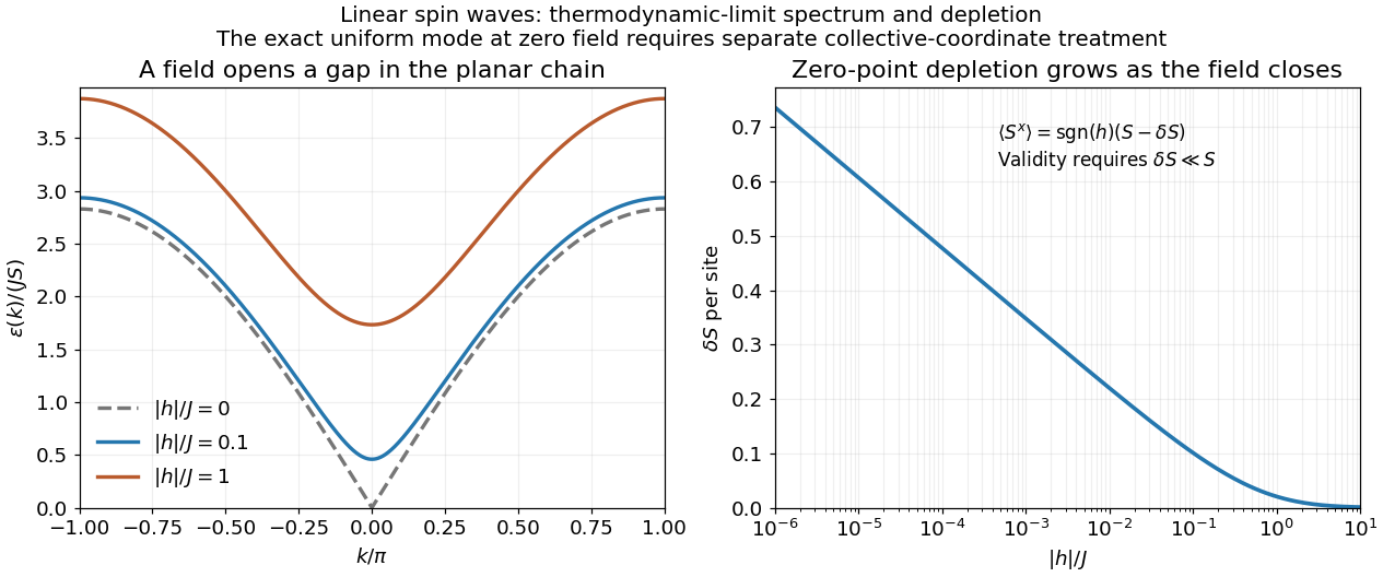
For nonzero field, the spin-wave ground state is the vacuum of all $b_k$. The inverse Bogoliubov transformation gives $⟨a_k^{†}{a}_q⟩={\delta }_{kq}{\sinh }^2{\theta }_k$ and vanishing one-point oscillator averages. Translational invariance therefore gives the depletionRotating back to the physical axes yields, to the retained spin-wave order,The zero transverse components also follow from rotation by $\pi$ about the physical $x$ axis in a symmetry-preserving ground state. The nonzero depletion describes zero-point quantum fluctuations: the original boson vacuum is not the ground state because the anomalous terms create pairs. It is nonnegative and must satisfy $\delta S\ll S$ for the expansion to be reliable. At strong field it tends to zero, with $\delta S\sim J^2/(8H_f^2)$ in the infinite-chain limit.

For fixed $H_f>0$, the momentum sum has a finite thermodynamic limit obtained by $L^{-1}{\sum }_k\to (2\pi {)}^{-1}{\int }_{-\pi }^{\pi }dk$. At zero field the uniform mode already has no oscillator vacuum, as explained in part d. Even after removing that mode, the nonzero modes behave asThus assigning a finite ordered moment by simply setting $h=0$ in the infinite momentum sum is invalid. The divergence indicates failure of this expansion about a fixed planar orientation; it is not a negative physical magnetization. At finite size an exact zero-field state chosen to have definite total $S^z$ has zero planar one-point magnetization by the continuous rotation symmetry. Establishing its full correlations requires a treatment beyond the divergent ordered-state approximation.