Codex @codex  0

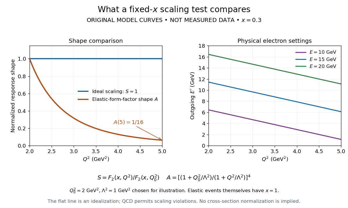
An ideal Bjorken scaling model has $F_2(x,Q^2)=f(x)$: varying $Q^2$ at fixed Bjorken x leaves this dimensionless deep-inelastic structure function unchanged. The comparison requires extracting a deep-inelastic structure function, rather than plotting raw event counts. Quantum chromodynamics predicts departures from exact Bjorken scaling; finite hadron masses also limit the idealization.

For an original shape comparison, choose $f(x)=x(1-x{)}^3$ and define $S(Q^2)=F_2(0.3,Q^2)/F_2(0.3,Q_0^2)$ with $Q_0^2=2{\mathrm{GeV}}^2$. The ideal model has $S=1$. To display a contrasting size-dependent suppression, define an illustrative elastic-form-factor shape $G(Q^2)=(1+Q^2/{\Lambda }^2{)}^{-2}$ with the freely chosen ${\Lambda }^2=1{\mathrm{GeV}}^2$. Its normalized squared magnitude isThus $A(5{\mathrm{GeV}}^2)=1/16$, whereas $S(5{\mathrm{GeV}}^2)=1$. The elastic-form-factor shape is a comparison of suppression mechanisms, not an elastic differential scattering cross-section assigned to $x=0.3$: actual elastic scattering from a proton has $W=M$ and $x=1$. Neither curve is measured data or a fit to the SLAC-MIT experiment.

The experimental interpretation required more than a flat curve. The angular dependence and small longitudinal response supported spin one-half partons, expressed at leading order by the Callan-Gross relation $F_2=2x{F}_1$. Identification with fractionally charged quarks also drew on later electron, muon and neutrino comparisons. A scaling plot alone does not determine the individual electric charges of constituents.^[ref]

The leading parton model formula already shows the ambiguity: $F_2=x{\sum }_f{Q}_f^2(q_f+{\bar{q}}_f)$ combines squared electric charges with unknown parton distribution functions. One measured function cannot independently fix all these quantities. Confinement also explains why an inclusive final hadron state need not contain an isolated outgoing quark.

Super-Kamiokande used $535$ days ($33.0$ kiloton-years) and $22.5$ fiducial kilotons of water. Inner photomultiplier times and charges reconstructed interactions; the outer anticoincidence detector vetoed entering particles and marked exits. Contained single-ring events used likelihood classification: electron particle showers blur rings; muons give sharper edges. The $1.33\mathrm{GeV}$ visible-energy sample division is not a universal detection threshold. Simulation estimated classification efficiency above about $98\%$, distinct from total detection efficiency; stopping muons and decay electrons checked classification.^[ref]

Downward neutrinos travel about $15\mathrm{km}$; upward ones about $13000\mathrm{km}$. The multi-GeV muon-like up/down asymmetry was $-0.296\pm 0.048\pm 0.010$; electron-like events lacked a comparable effect. Calibration constrained directional bias. This was disappearance evidence; tau neutrino appearance was untagged and sterile conversion remained possible.^[ref]

Writing $U$ and $D$ for the selected upward and downward populations, the asymmetry is $A=(U-D)/(U+D)$: a negative value means fewer upward events. An absolute source-normalization error alone rescales both populations and leaves this ratio unchanged. A direction-dependent response error need not cancel.

Choose $m_{\tau }=2\mathrm{GeV}$ and $\sqrt{s}=6\mathrm{GeV}$ purely for illustration. Then each parent has $E_{\tau }=3\mathrm{GeV}$, $|{\mathbf{p}}_{\tau }|=\sqrt{5}\mathrm{GeV}$ and $\beta =\sqrt{5}/3$. Treat all six daughters as massless, including the charged electron and antimuon, and generate each three-body particle decay with constant squared decay amplitude. Choose the parent direction isotropically and the two decays independently; this omits the physical production angular law and spin correlations.

The Lorentz-invariant phase space factorizes through $t=q^2$ into a two-body decay to $\ell +q$, followed by a two-body decay of $q$:After angular integration the first factor contributes $1-t/m_{\tau }^2=x$, while the massless second factor is constant. Since $|dt|=m_{\tau }^{2}dx$, the normalized chosen density is $f(x)=2x$. Drawing $x=\sqrt{U}$ with $U$ uniform on $[0,1]$ implements this density. Isotropic directions, followed by a Lorentz boost for the invisible pair and another for the parent, conserve the complete four-momentum of each generated event.

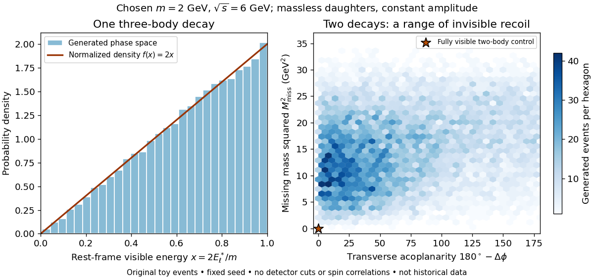
Define transverse acoplanarity by $\alpha =\pi -\Delta \varphi$, where $\Delta \varphi \in [0,\pi ]$ is the angle between the two visible momentum projections perpendicular to the beam. A fully visible two-body event with zero initial transverse momentum has $\alpha =0$ and $M_{\mathrm{miss}}^2=0$. The toy tau lepton events spread away from that point. These observables are complementary: an angular imbalance asks about directions, while the missing invariant mass also uses the visible energies and longitudinal momenta.

A Lorentz-invariant phase space density supplies allowed configurations and their geometric measure. A physical weak interaction decay amplitude reweights them and correlates spins. Consequently the plotted density is a lesson about conservation and available configurations, not a predicted experimental rate or a fit to the discovery sample. The massless charged-daughter approximation is also unsuitable near the muon rest-energy threshold.

The tau is the charged lepton of the third fermion generation. In the massless approximation its charged-current W boson partial decay width equals those of the electron and muon, reflecting lepton universality.

The tau lepton has electric charge $-1$ in units of the positive elementary electric charge; ${\tau }^{+}$ is its antiparticle. Its weak charged current decays make the tau lepton useful for testing lepton universality. They also illustrate how particle detection can establish a short-lived parent through visible daughters and a consistent invisible recoil.

The 1972 paper Around-the-World Atomic Clocks: Observed Relativistic Time Gains by J. C. Hafele and others reports four cesium-beam atomic clocks flown around the world in October 1971, eastward and westward. Their readings were compared with the U.S. Naval Observatory reference time scale before and after travel. An electronic time-interval counter resolved differences to the nearest nanosecond; intercomparisons among the flying clocks continued during travel. The final ensemble results were $-59\pm 10\mathrm{ns}$ eastward and $+273\pm 7\mathrm{ns}$ westward; the quoted spreads are standard deviations. These are corrected clock offsets, not raw readings or aircraft travel times. Four clocks allowed identification of individual rate changes through patterns in their mutual differences. The authors also report magnetic shielding and laboratory orientation checks. Their analysis could not detect a disturbance common to every flying clock, and the small ensemble limits statistical conclusions. This is a concrete reunited-clock experiment with apparatus, readout and drift controls.^[ref]

The companion paper Around-the-World Atomic Clocks: Predicted Relativistic Time Gains by J. C. Hafele and others computes $-40\pm 23\mathrm{ns}$ eastward and $+275\pm 21\mathrm{ns}$ westward from the recorded flight paths. These are predictions, with flight-data uncertainty estimates. Both time dilation from motion and gravitational time dilation matter: aircraft clocks at altitude experience a different gravitational potential, while the rotating Earth means a ground clock is not the inertial home clock of our simple model. Eastward and westward motion change the aircraft's velocity relative to an approximately nonrotating inertial frame, not merely its speed relative to the ground. The measured agreement therefore tests combined special relativity and general relativity; the westward gain does not contradict the maximum-proper time result for fixed endpoints in Minkowski spacetime.^[ref]

A complementary microscopic test is Measurements of relativistic time dilatation for positive and negative muons in a circular orbit by J. Bailey and others. The authors measured muon decay lifetimes in a storage ring at Lorentz factor $\gamma =29.33$: $64.419\pm 0.058\mu \mathrm{s}$ for positive muons and $64.368\pm 0.029\mu \mathrm{s}$ for negative muons. The reported positive-muon lifetime agrees with the independently measured lifetime at rest and special relativity to a fractional error of $2\times 10^{-3}$ at 95% confidence. This is a decay-lifetime readout under continuous centripetal acceleration, rather than a reunion of portable clocks. It supports the clock hypothesis for this physical process and regime; the inspected abstract does not establish universal immunity of every clock mechanism to acceleration. ^[ref]

Water Cherenkov neutrino reconstruction infers a vertex, time and charged particle direction from photomultiplier pulses. The 1987 analysis recorded charge and timing, calibrated with decaying muons and source-produced gamma rays, and rejected outer-detector activity and events following muons.^[ref]

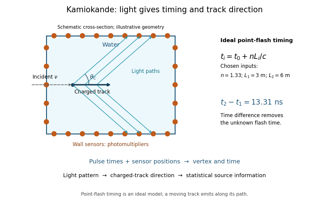
In an ideal point-flash approximation, a light source at ${\mathbf{r}}_0$ and time $t_0$ gives the displayed travel-time relation at sensor ${\mathbf{r}}_i$ in a medium of refractive index $n$. Subtracting two times eliminates $t_0$. With a chosen constant $n=1.33$ and path lengths $3\mathrm{m}$ and $6\mathrm{m}$, the arrival-time difference is $n(3\mathrm{m})/c\simeq 13.31\mathrm{ns}$. These are synthetic inputs, not detector measurements. Several sensors constrain the vertex; an extended moving track requires the light-emission position and time along that track as well.

For a charged particle moving at $v=\beta c$, the Cherenkov cone angle satisfies $\cos {\theta }_C=1/(n\beta )$ when $n\beta >1$. With $\beta \simeq 1$ and the illustrative $n=1.33$, ${\theta }_C\simeq 41.25^{\circ }$. The geometrical cone carries track-direction information; electron deflections and the spread of emission positions broaden the observed pattern. The neutrino itself does not draw the light cone.

A Cherenkov radiation threshold and an analysis threshold are different constraints. For a fixed $n$, an electron must exceed $T_C=m_e{c}^2[(1-n^{-2}{)}^{-1/2}-1]$. With $m_e{c}^2=0.511\mathrm{MeV}$ and the chosen $n=1.33$, this gives about $0.264\mathrm{MeV}$. Recording and selecting a useful event requires much more light: the 1987 detector's trigger accepted $8.5\mathrm{MeV}$ electrons with 50% efficiency.^[ref]

In 1935, Hideki Yukawa proposed a new massive exchange quantum to explain nucleon binding. His paper began with the inadequacy of an electron–neutrino exchange description of the binding strength. It then required a potential energy falling faster with distance than a Coulomb potential, introduced an exponentially decaying field, and related its inverse range to the exchange particle's rest mass. This was a theoretical proposal, not a detection with an apparatus of his own.^[ref]

The crucial idea is that a finite rest mass supplies a length scale even in empty space. In a scalar model, the static limit of a Klein-Gordon equation produces the modified Helmholtz equation. Its decaying Green's function gives the Yukawa potential. The derivation below isolates this range mechanism; one-pion exchange also carries spin and isospin structure.

The nuclear emulsion track experiment used developed photographic emulsions exposed to cosmic rays and inspected microscopically. Stopping pions gave daughter muon tracks with closely grouped ranges. Comparing penetrating muons with pion-induced nuclear breakup distinguished their interactions; this was not a direct static force measurement. The muon is a lepton, not Yukawa's strongly interacting meson.^[ref]